Transient diffusion - partial differential equations

| categories: pde | tags: mass transfer

We want to solve for the concentration profile of component that diffuses into a 1D rod, with an impermeable barrier at the end. The PDE governing this situation is:

\(\frac{\partial C}{\partial t} = D \frac{\partial^2 C}{\partial x^2}\)

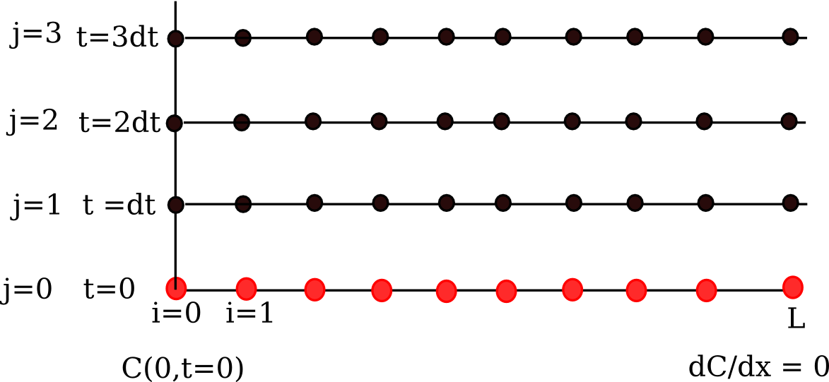
at \(t=0\), in this example we have \(C_0(x) = 0\) as an initial condition, with boundary conditions \(C(0,t)=0.1\) and \(\partial C/ \partial x(L,t)=0\).

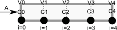
We are going to discretize this equation in both time and space to arrive at the solution. We will let \(i\) be the index for the spatial discretization, and \(j\) be the index for the temporal discretization. The discretization looks like this.

Note that we cannot use the method of lines as we did before because we have the derivative-based boundary condition at one of the boundaries.

We approximate the time derivative as:

\(\frac{\partial C}{\partial t} \bigg| _{i,j} \approx \frac{C_{i,j+1} - C_{i,j}}{\Delta t} \)

\(\frac{\partial^2 C}{\partial x^2} \bigg| _{i,j} \approx \frac{C_{i+1,j} - 2 C_{i,j} + C_{i-1,j}}{h^2} \)

We define \(\alpha = \frac{D \Delta t}{h^2}\), and from these two approximations and the PDE, we solve for the unknown solution at a later time step as:

\(C_{i, j+1} = \alpha C_{i+1,j} + (1 - 2 \alpha) C_{i,j} + \alpha C_{i-1,j} \)

We know \(C_{i,j=0}\) from the initial conditions, so we simply need to iterate to evaluate \(C_{i,j}\), which is the solution at each time step.

See also: http://www3.nd.edu/~jjwteach/441/PdfNotes/lecture16.pdf

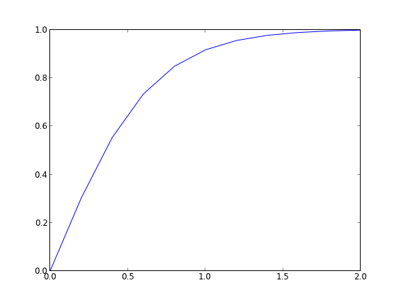
import numpy as np
import matplotlib.pyplot as plt

N = 20  # number of points to discretize
L = 1.0
X = np.linspace(0, L, N) # position along the rod
h = L / (N - 1)          # discretization spacing

C0t = 0.1  # concentration at x = 0
D = 0.02

tfinal = 50.0
Ntsteps = 1000
dt = tfinal / (Ntsteps - 1)
t = np.linspace(0, tfinal, Ntsteps)

alpha = D * dt / h**2
print alpha

C_xt = [] # container for all the time steps

# initial condition at t = 0
C = np.zeros(X.shape)
C[0] = C0t

C_xt += [C]

for j in range(1, Ntsteps):
    N = np.zeros(C.shape)
    N[0] =  C0t
    N[1:-1] = alpha*C[2:] + (1 - 2 * alpha) * C[1:-1] + alpha * C[0:-2]
    N[-1] = N[-2]  # derivative boundary condition flux = 0
    C[:] = N
    C_xt += [N]

    # plot selective solutions
    if j in [1,2,5,10,20,50,100,200,500]:
        plt.plot(X, N, label='t={0:1.2f}'.format(t[j]))

plt.xlabel('Position in rod')
plt.ylabel('Concentration')
plt.title('Concentration at different times')
plt.legend(loc='best')
plt.savefig('images/transient-diffusion-temporal-dependence.png')

C_xt = np.array(C_xt)
plt.figure()
plt.plot(t, C_xt[:,5], label='x={0:1.2f}'.format(X[5]))
plt.plot(t, C_xt[:,10], label='x={0:1.2f}'.format(X[10]))
plt.plot(t, C_xt[:,15], label='x={0:1.2f}'.format(X[15]))
plt.plot(t, C_xt[:,19], label='x={0:1.2f}'.format(X[19]))
plt.legend(loc='best')
plt.xlabel('Time')
plt.ylabel('Concentration')
plt.savefig('images/transient-diffusion-position-dependence.png')

plt.show()
0.361361361361

The solution is somewhat sensitive to the choices of time step and spatial discretization. If you make the time step too big, the method is not stable, and large oscillations may occur.

Copyright (C) 2013 by John Kitchin. See the License for information about copying.

org-mode source

Discuss on Twitter

A nonlinear BVP

| categories: pde | tags:

Adapted from Example 8.7 in _Numerical Methods in Engineering with Python_ by Jaan Kiusalaas.

We want to solve \(y''(x) = -3 y(x) y'(x)\) with $y(0) = 0 and \(y(2) = 1\) using a finite difference method. We discretize the region and approximate the derivatives as:

\(y''(x) \approx \frac{y_{i-1} - 2 y_i + y_{i+1}}{h^2} \)

\(y'(x) \approx \frac{y_{i+1} - y_{i-1}}{2 h} \)

We define a function \(y''(x) = F(x, y, y')\). At each node in our discretized region, we will have an equation that looks like \(y''(x) - F(x, y, y') = 0\), which will be nonlinear in the unknown solution \(y\). The set of equations to solve is:

\begin{eqnarray} y_0 - \alpha &=& 0 \\ \frac{y_{i-1} - 2 y_i + y_{i+1}}{h^2} + (3 y_i) (\frac{y_{i+1} - y_{i-1}}{2 h}) &=& 0 \\ y_L - \beta &=&0 \end{eqnarray}

Since we use a nonlinear solver, we will have to provide an initial guess to the solution. We will in this case assume a line. In other cases, a bad initial guess may lead to no solution.

import numpy as np
from scipy.optimize import fsolve
import matplotlib.pyplot as plt

x1 = 0.0
x2 = 2.0

alpha = 0.0
beta = 1.0

N = 11
X = np.linspace(x1, x2, N)
h = (x2 - x1) / (N - 1)

def Ypp(x, y, yprime):
    '''define y'' = 3*y*y' '''
    return -3.0 * y * yprime

def residuals(y):
    '''When we have the right values of y, this function will be zero.'''

    res = np.zeros(y.shape)

    res[0] = y[0] - alpha
    
    for i in range(1, N - 1):
        x = X[i]
        YPP = (y[i - 1] - 2 * y[i] + y[i + 1]) / h**2
        YP = (y[i + 1] - y[i - 1]) / (2 * h)
        res[i] = YPP - Ypp(x, y[i], YP)

    res[-1] = y[-1] - beta
    return res

# we need an initial guess
init = alpha + (beta - alpha) / (x2 - x1) * X

Y = fsolve(residuals, init)

plt.plot(X, Y)
plt.savefig('images/bvp-nonlinear-1.png')

That code looks useful, so I put it in the pycse module in the function BVP_nl. Here is an example usage. We have to create two functions, one for the differential equation, and one for the initial guess.

from pycse import  BVP_nl
import matplotlib.pyplot as plt

def Ypp(x, y, yprime):
    '''define y'' = 3*y*y' '''
    return -3.0 * y * yprime

def init(x):
    return alpha + (beta - alpha) / (x2 - x1) * x

x1 = 0.0
x2 = 2.0

alpha = 0.0
beta = 1.0

N = 11
x, y = BVP_nl(Ypp, x1, x2, alpha, beta, init, N)

plt.plot(x, y)
plt.savefig('images/bvp-nonlinear-2.png')

The results are the same.

Copyright (C) 2013 by John Kitchin. See the License for information about copying.

org-mode source

Discuss on Twitter

Transient heat conduction - partial differential equations

| categories: pde | tags: heat transfer

Matlab post adapated from http://msemac.redwoods.edu/~darnold/math55/DEproj/sp02/AbeRichards/slideshowdefinal.pdf

We solved a steady state BVP modeling heat conduction. Today we examine the transient behavior of a rod at constant T put between two heat reservoirs at different temperatures, again T1 = 100, and T2 = 200. The rod will start at 150. Over time, we should expect a solution that approaches the steady state solution: a linear temperature profile from one side of the rod to the other.

\(\frac{\partial u}{\partial t} = k \frac{\partial^2 u}{\partial x^2}\)

at \(t=0\), in this example we have \(u_0(x) = 150\) as an initial condition. with boundary conditions \(u(0,t)=100\) and \(u(L,t)=200\).

In Matlab there is the pdepe command. There is not yet a PDE solver in scipy. Instead, we will utilze the method of lines to solve this problem. We discretize the rod into segments, and approximate the second derivative in the spatial dimension as \(\frac{\partial^2 u}{\partial x^2} = (u(x + h) - 2 u(x) + u(x-h))/ h^2\) at each node. This leads to a set of coupled ordinary differential equations that is easy to solve.

Let us say the rod has a length of 1, \(k=0.02\), and solve for the time-dependent temperature profiles.

import numpy as np
from scipy.integrate import odeint
import matplotlib.pyplot as plt

N = 100  # number of points to discretize
L = 1.0
X = np.linspace(0, L, N) # position along the rod
h = L / (N - 1)

k = 0.02

def odefunc(u, t):
    dudt = np.zeros(X.shape)

    dudt[0] = 0 # constant at boundary condition
    dudt[-1] = 0

    # now for the internal nodes
    for i in range(1, N-1):
        dudt[i] = k * (u[i + 1] - 2*u[i] + u[i - 1]) / h**2

    return dudt

init = 150.0 * np.ones(X.shape) # initial temperature
init[0] = 100.0  # one boundary condition
init[-1] = 200.0 # the other boundary condition

tspan = np.linspace(0.0, 5.0, 100)
sol = odeint(odefunc, init, tspan)


for i in range(0, len(tspan), 5):
    plt.plot(X, sol[i], label='t={0:1.2f}'.format(tspan[i]))

# put legend outside the figure
plt.legend(loc='center left', bbox_to_anchor=(1, 0.5))
plt.xlabel('X position')
plt.ylabel('Temperature')

# adjust figure edges so the legend is in the figure
plt.subplots_adjust(top=0.89, right=0.77)
plt.savefig('images/pde-transient-heat-1.png')


# Make a 3d figure
from mpl_toolkits.mplot3d import Axes3D
fig = plt.figure()
ax = fig.add_subplot(111, projection='3d')

SX, ST = np.meshgrid(X, tspan)
ax.plot_surface(SX, ST, sol, cmap='jet')
ax.set_xlabel('X')
ax.set_ylabel('time')
ax.set_zlabel('T')
ax.view_init(elev=15, azim=-124) # adjust view so it is easy to see
plt.savefig('images/pde-transient-heat-3d.png')

# animated solution. We will use imagemagick for this

# we save each frame as an image, and use the imagemagick convert command to 
# make an animated gif
for i in range(len(tspan)):
    plt.clf()
    plt.plot(X, sol[i])
    plt.xlabel('X')
    plt.ylabel('T(X)')
    plt.title('t = {0}'.format(tspan[i]))
    plt.savefig('___t{0:03d}.png'.format(i))

import commands
print commands.getoutput('convert -quality 100 ___t*.png images/transient_heat.gif')
print commands.getoutput('rm ___t*.png') #remove temp files


This version of the graphical solution is not that easy to read, although with some study you can see the solution evolves from the initial condition which is flat, to the steady state solution which is a linear temperature ramp.

The 3d version may be easier to interpret. The temperature profile starts out flat, and gradually changes to the linear ramp.

Finally, the animated solution.

Copyright (C) 2013 by John Kitchin. See the License for information about copying.

org-mode source

Discuss on Twitter

Modeling a transient plug flow reactor

| categories: animation, pde | tags: reaction engineering

Matlab post

The PDE that describes the transient behavior of a plug flow reactor with constant volumetric flow rate is:

\( \frac{\partial C_A}{\partial dt} = -\nu_0 \frac{\partial C_A}{\partial dV} + r_A \).

To solve this numerically in python, we will utilize the method of lines. The idea is to discretize the reactor in volume, and approximate the spatial derivatives by finite differences. Then we will have a set of coupled ordinary differential equations that can be solved in the usual way. Let us simplify the notation with \(C = C_A\), and let \(r_A = -k C^2\). Graphically this looks like this:

This leads to the following set of equations:

\begin{eqnarray} \frac{dC_0}{dt} &=& 0 \text{ (entrance concentration never changes)} \\ \frac{dC_1}{dt} &=& -\nu_0 \frac{C_1 - C_0}{V_1 - V_0} - k C_1^2 \\ \frac{dC_2}{dt} &=& -\nu_0 \frac{C_2 - C_1}{V_2 - V_1} - k C_2^2 \\ \vdots \\ \frac{dC_4}{dt} &=& -\nu_0 \frac{C_4 - C_3}{V_4 - V_3} - k C_4^2 \end{eqnarray}

Last, we need initial conditions for all the nodes in the discretization. Let us assume the reactor was full of empty solvent, so that \(C_i = 0\) at \(t=0\). In the next block of code, we get the transient solutions, and the steady state solution.

import numpy as np
from scipy.integrate import odeint

Ca0 = 2     # Entering concentration
vo = 2      # volumetric flow rate
volume = 20 # total volume of reactor, spacetime = 10
k = 1       # reaction rate constant

N = 100     # number of points to discretize the reactor volume on

init = np.zeros(N)    # Concentration in reactor at t = 0
init[0] = Ca0         # concentration at entrance

V = np.linspace(0, volume, N) # discretized volume elements
tspan = np.linspace(0, 25)    # time span to integrate over

def method_of_lines(C, t):
    'coupled ODES at each node point'
    D = -vo * np.diff(C) / np.diff(V) - k * C[1:]**2
    return np.concatenate([[0], #C0 is constant at entrance
                            D])


sol = odeint(method_of_lines, init, tspan)

# steady state solution
def pfr(C, V):
    return 1.0 / vo * (-k * C**2)

ssol = odeint(pfr, Ca0, V)

The transient solution contains the time dependent behavior of each node in the discretized reactor. Each row contains the concentration as a function of volume at a specific time point. For example, we can plot the concentration of A at the exit vs. time (that is, the last entry of each row) as:

import matplotlib.pyplot as plt
plt.plot(tspan, sol[:, -1])
plt.xlabel('time')
plt.ylabel('$C_A$ at exit')
plt.savefig('images/transient-pfr-1.png')
[<matplotlib.lines.Line2D object at 0x05A18830>]
<matplotlib.text.Text object at 0x059FE1D0>
<matplotlib.text.Text object at 0x05A05270>

After approximately one space time, the steady state solution is reached at the exit. For completeness, we also examine the steady state solution.

plt.figure()
plt.plot(V, ssol, label='Steady state')
plt.plot(V, sol[-1], label='t = {}'.format(tspan[-1]))
plt.xlabel('Volume')
plt.ylabel('$C_A$')
plt.legend(loc='best')
plt.savefig('images/transient-pfr-2.png')

There is some minor disagreement between the final transient solution and the steady state solution. That is due to the approximation in discretizing the reactor volume. In this example we used 100 nodes. You get better agreement with a larger number of nodes, say 200 or more. Of course, it takes slightly longer to compute then, since the number of coupled odes is equal to the number of nodes.

We can also create an animated gif to show how the concentration of A throughout the reactor varies with time. Note, I had to install ffmpeg (http://ffmpeg.org/) to save the animation.

from matplotlib import animation

# make empty figure
fig = plt.figure()
ax = plt.axes(xlim=(0, 20), ylim=(0, 2))
line, = ax.plot(V, init, lw=2)

def animate(i):
    line.set_xdata(V)
    line.set_ydata(sol[i])
    ax.set_title('t = {0}'.format(tspan[i]))
    ax.figure.canvas.draw() 
    return line,
    

anim = animation.FuncAnimation(fig, animate, frames=50,  blit=True)

anim.save('images/transient_pfr.mp4', fps=10)

http://jkitchin.github.com/media/transient_pfr.mp4

You can see from the animation that after about 10 time units, the solution is not changing further, suggesting steady state has been reached.

Copyright (C) 2013 by John Kitchin. See the License for information about copying.

org-mode source

Discuss on Twitter