Fit a line to numerical data

| categories: data analysis | tags:

Matlab post

We want to fit a line to this data:

x = [0, 0.5, 1, 1.5, 2.0, 3.0, 4.0, 6.0, 10]
y = [0, -0.157, -0.315, -0.472, -0.629, -0.942, -1.255, -1.884, -3.147]

We use the polyfit(x, y, n) command where n is the polynomial order, n=1 for a line.

import numpy as np

p = np.polyfit(x, y, 1)
print p
slope, intercept = p
print slope, intercept
>>> >>> [-0.31452218  0.00062457]
>>> -0.3145221843 0.00062457337884

To show the fit, we can use numpy.polyval to evaluate the fit at many points.

import matplotlib.pyplot as plt

xfit = np.linspace(0, 10)
yfit = np.polyval(p, xfit)

plt.plot(x, y, 'bo', label='raw data')
plt.plot(xfit, yfit, 'r-', label='fit')
plt.xlabel('x')
plt.ylabel('y')
plt.legend()
plt.savefig('images/linefit-1.png')
>>> >>> >>> >>> [<matplotlib.lines.Line2D object at 0x053C1790>]
[<matplotlib.lines.Line2D object at 0x0313C610>]
<matplotlib.text.Text object at 0x052A4950>
<matplotlib.text.Text object at 0x052B9A10>
<matplotlib.legend.Legend object at 0x053C1CD0>

Copyright (C) 2013 by John Kitchin. See the License for information about copying.

org-mode source

Discuss on Twitter

Random thoughts

| categories: statistics, math | tags:

Matlab post

Random numbers are used in a variety of simulation methods, most notably Monte Carlo simulations. In another later example, we will see how we can use random numbers for error propagation analysis. First, we discuss two types of pseudorandom numbers we can use in python: uniformly distributed and normally distributed numbers.

Say you are the gambling type, and bet your friend $5 the next random number will be greater than 0.49. Let us ask Python to roll the random number generator for us.

import numpy as np

n = np.random.uniform()
print 'n = {0}'.format(n)

if n > 0.49:
    print 'You win!'
else:
    print 'you lose.'
n = 0.381896986693
you lose.

The odds of you winning the last bet are slightly stacked in your favor. There is only a 49% chance your friend wins, but a 51% chance that you win. Lets play the game a lot of times times and see how many times you win, and your friend wins. First, lets generate a bunch of numbers and look at the distribution with a histogram.

import numpy as np

N = 10000
games = np.random.uniform(size=(1,N))

wins = np.sum(games > 0.49)
losses = N - wins

print 'You won {0} times ({1:%})'.format(wins, float(wins) / N)

import matplotlib.pyplot as plt
count, bins, ignored = plt.hist(games)
plt.savefig('images/random-thoughts-1.png')
You won 5090 times (50.900000%)

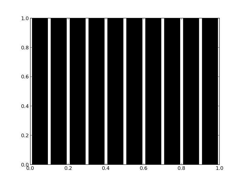
As you can see you win slightly more than you lost.

It is possible to get random integers. Here are a few examples of getting a random integer between 1 and 100. You might do this to get random indices of a list, for example.

import numpy as np

print np.random.random_integers(1, 100)
print np.random.random_integers(1, 100, 3)
print np.random.random_integers(1, 100, (2,2))
96
[ 95  49 100]
[[69 54]
 [41 93]]

The normal distribution is defined by \(f(x)=\frac{1}{\sqrt{2\pi \sigma^2}} \exp (-\frac{(x-\mu)^2}{2\sigma^2})\) where \(\mu\) is the mean value, and \(\sigma\) is the standard deviation. In the standard distribution, \(\mu=0\) and \(\sigma=1\).

import numpy as np

mu = 1
sigma = 0.5
print np.random.normal(mu, sigma)
print np.random.normal(mu, sigma, 2)
1.04225842065
[ 0.58105204  0.64853157]

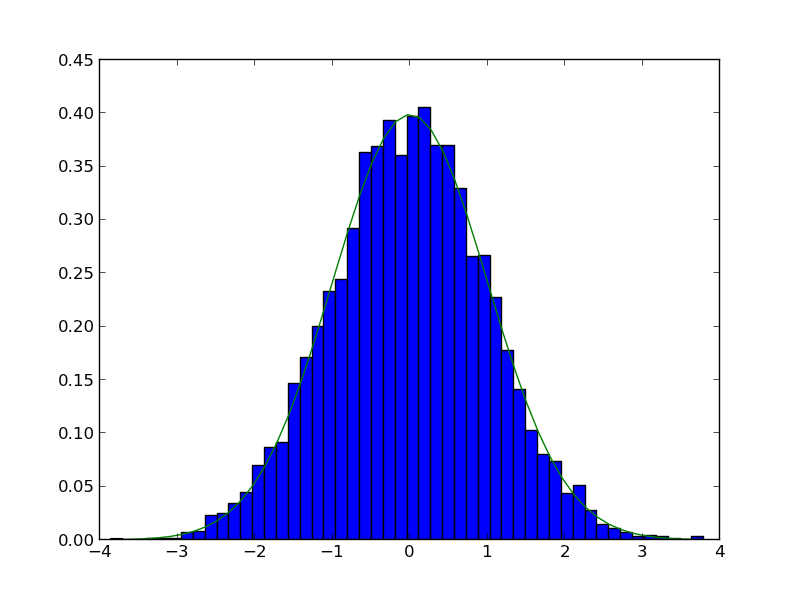
Let us compare the sampled distribution to the analytical distribution. We generate a large set of samples, and calculate the probability of getting each value using the matplotlib.pyplot.hist command.

import numpy as np
import matplotlib.pyplot as plt

mu = 0; sigma = 1

N = 5000
samples = np.random.normal(mu, sigma, N)

counts, bins, ignored = plt.hist(samples, 50, normed=True)

plt.plot(bins, 1.0/np.sqrt(2 * np.pi * sigma**2)*np.exp(-((bins - mu)**2)/(2*sigma**2)))
plt.savefig('images/random-thoughts-2.png')

What fraction of points lie between plus and minus one standard deviation of the mean?

samples >= mu-sigma will return a vector of ones where the inequality is true, and zeros where it is not. (samples >= mu-sigma) & (samples <= mu+sigma) will return a vector of ones where there is a one in both vectors, and a zero where there is not. In other words, a vector where both inequalities are true. Finally, we can sum the vector to get the number of elements where the two inequalities are true, and finally normalize by the total number of samples to get the fraction of samples that are greater than -sigma and less than sigma.

import numpy as np
import matplotlib.pyplot as plt

mu = 0; sigma = 1

N = 5000
samples = np.random.normal(mu, sigma, N)

a = np.sum((samples >= (mu - sigma)) & (samples <= (mu + sigma))) / float(N) 
b = np.sum((samples >= (mu - 2*sigma)) & (samples <= (mu + 2*sigma))) / float(N) 
print '{0:%} of samples are within +- standard deviations of the mean'.format(a)
print '{0:%} of samples are within +- 2standard deviations of the mean'.format(b)
67.500000% of samples are within +- standard deviations of the mean
95.580000% of samples are within +- 2standard deviations of the mean

1 Summary

We only considered the numpy.random functions here, and not all of them. There are many distributions of random numbers to choose from. There are also random numbers in the python random module. Remember these are only pseudorandom numbers, but they are still useful for many applications.

Copyright (C) 2013 by John Kitchin. See the License for information about copying.

org-mode source

Discuss on Twitter

Calculating a bubble point pressure of a mixture

| categories: nonlinear algebra | tags: thermodynamics

Matlab post

Adapted from http://terpconnect.umd.edu/~nsw/ench250/bubpnt.htm (dead link)

We previously learned to read a datafile containing lots of Antoine coefficients into a database, and use the coefficients to estimate vapor pressure of a single compound. Here we use those coefficents to compute a bubble point pressure of a mixture.

The bubble point is the temperature at which the sum of the component vapor pressures is equal to the the total pressure. This is where a bubble of vapor will first start forming, and the mixture starts to boil.

Consider an equimolar mixture of benzene, toluene, chloroform, acetone and methanol. Compute the bubble point at 760 mmHg, and the gas phase composition. The gas phase composition is given by: \(y_i = x_i*P_i/P_T\).

import numpy as np
from scipy.optimize import fsolve

# load our thermodynamic data
data = np.loadtxt('data/antoine_data.dat',
                  dtype=[('id', np.int),
                         ('formula', 'S8'),
                         ('name', 'S28'),
                         ('A', np.float),
                         ('B', np.float),
                         ('C', np.float),
                         ('Tmin', np.float),
                         ('Tmax', np.float),
                         ('??', 'S4'),
                         ('?', 'S4')],
                  skiprows=7)

compounds = ['benzene', 'toluene', 'chloroform', 'acetone', 'methanol']

# extract the data we want
A = np.array([data[data['name'] == x]['A'][0] for x in compounds])
B = np.array([data[data['name'] == x]['B'][0] for x in compounds])
C = np.array([data[data['name'] == x]['C'][0] for x in compounds])
Tmin = np.array([data[data['name'] == x]['Tmin'][0] for x in compounds])
Tmax = np.array([data[data['name'] == x]['Tmax'][0] for x in compounds])


# we have an equimolar mixture
x = np.array([0.2, 0.2, 0.2, 0.2, 0.2])

# Given a T, we can compute the pressure of each species like this:

T = 67 # degC
P = 10**(A - B / (T + C))
print P
print np.dot(x, P)  # total mole-fraction weighted pressure

Tguess = 67
Ptotal = 760

def func(T):
    P = 10**(A - B / (T + C))
    return Ptotal - np.dot(x, P)
    
Tbubble, = fsolve(func, Tguess)

print 'The bubble point is {0:1.2f} degC'.format(Tbubble)

# double check answer is in a valid T range
if np.any(Tbubble < Tmin) or np.any(Tbubble > Tmax):
    print 'T_bubble is out of range!'

# print gas phase composition
y = x * 10**(A - B / (Tbubble + C))/Ptotal

for cmpd, yi in zip(compounds, y):
    print 'y_{0:<10s} = {1:1.3f}'.format(cmpd, yi)
[  498.4320267    182.16010994   898.31061294  1081.48181768   837.88860027]
699.654633507
The bubble point is 69.46 degC
y_benzene    = 0.142
y_toluene    = 0.053
y_chloroform = 0.255
y_acetone    = 0.308
y_methanol   = 0.242

Copyright (C) 2013 by John Kitchin. See the License for information about copying.

org-mode source

Discuss on Twitter

Parameter estimation by directly minimizing summed squared errors

| categories: data analysis | tags:

Matlab post

import numpy as np
import matplotlib.pyplot as plt

x = np.array([0.0,       1.1,       2.3,      3.1,       4.05,      6.0])
y = np.array([0.0039,    1.2270,    5.7035,   10.6472,   18.6032,   42.3024])

plt.plot(x, y)
plt.xlabel('x')
plt.ylabel('y')
plt.savefig('images/nonlin-minsse-1.png')
>>> >>> >>> >>> >>> [<matplotlib.lines.Line2D object at 0x000000000733D898>]
<matplotlib.text.Text object at 0x00000000071EC5C0>
<matplotlib.text.Text object at 0x00000000071EED30>

We are going to fit the function \(y = x^a\) to the data. The best \(a\) will minimize the summed squared error between the model and the fit.

def errfunc_(a):
    return np.sum((y - x**a)**2)

errfunc = np.vectorize(errfunc_)

arange = np.linspace(1, 3)
sse = errfunc(arange)

plt.figure()
plt.plot(arange, sse)
plt.xlabel('a')
plt.ylabel('$\Sigma (y - y_{pred})^2$')
plt.savefig('images/nonlin-minsse-2.png')
... >>> >>> >>> >>> >>> >>> <matplotlib.figure.Figure object at 0x000000000736DBA8>
[<matplotlib.lines.Line2D object at 0x00000000075CBEF0>]
<matplotlib.text.Text object at 0x00000000076B8C18>
<matplotlib.text.Text object at 0x0000000007698BE0>

Based on the graph above, you can see a minimum in the summed squared error near \(a = 2.1\). We use that as our initial guess. Since we know the answer is bounded, we use scipy.optimize.fminbound

from scipy.optimize import fminbound

amin = fminbound(errfunc, 1.0, 3.0)

print amin

plt.figure()
plt.plot(x, y, 'bo', label='data')
plt.plot(x, x**amin, 'r-', label='fit')
plt.xlabel('x')
plt.ylabel('y')
plt.legend(loc='best')
plt.savefig('images/nonlin-minsse-3.png')
>>> >>> >>> 2.09004838933
>>> <matplotlib.figure.Figure object at 0x00000000075D8470>
[<matplotlib.lines.Line2D object at 0x0000000007BDFA20>]
[<matplotlib.lines.Line2D object at 0x0000000007BDFC18>]
<matplotlib.text.Text object at 0x0000000007BC6828>
<matplotlib.text.Text object at 0x0000000007BCAF98>
<matplotlib.legend.Legend object at 0x0000000007BE3128>

We can do nonlinear fitting by directly minimizing the summed squared error between a model and data. This method lacks some of the features of other methods, notably the simple ability to get the confidence interval. However, this method is flexible and may offer more insight into how the solution depends on the parameters.

Copyright (C) 2013 by John Kitchin. See the License for information about copying.

org-mode source

Discuss on Twitter

Fitting a numerical ODE solution to data

| categories: data analysis, nonlinear regression | tags:

Matlab post

Suppose we know the concentration of A follows this differential equation: \(\frac{dC_A}{dt} = -k C_A\), and we have data we want to fit to it. Here is an example of doing that.

import numpy as np
from scipy.optimize import curve_fit
from scipy.integrate import odeint

# given data we want to fit
tspan = [0, 0.1, 0.2, 0.4, 0.8, 1]
Ca_data = [2.0081,  1.5512,  1.1903,  0.7160,  0.2562,  0.1495]

def fitfunc(t, k):
    'Function that returns Ca computed from an ODE for a k'
    def myode(Ca, t):
        return -k * Ca

    Ca0 = Ca_data[0]
    Casol = odeint(myode, Ca0, t)
    return Casol[:,0]

k_fit, kcov = curve_fit(fitfunc, tspan, Ca_data, p0=1.3)
print k_fit

tfit = np.linspace(0,1);
fit = fitfunc(tfit, k_fit)

import matplotlib.pyplot as plt
plt.plot(tspan, Ca_data, 'ro', label='data')
plt.plot(tfit, fit, 'b-', label='fit')
plt.legend(loc='best')
plt.savefig('images/ode-fit.png')
[ 2.58893455]

Copyright (C) 2013 by John Kitchin. See the License for information about copying.

org-mode source

Discuss on Twitter
« Previous Page -- Next Page »