The Kitchin Research Group: nonlinear regression

Fitting a numerical ODE solution to data

Posted February 18, 2013 at 09:00 AM | categories: nonlinear regression, data analysis | tags:

Updated February 27, 2013 at 02:39 PM

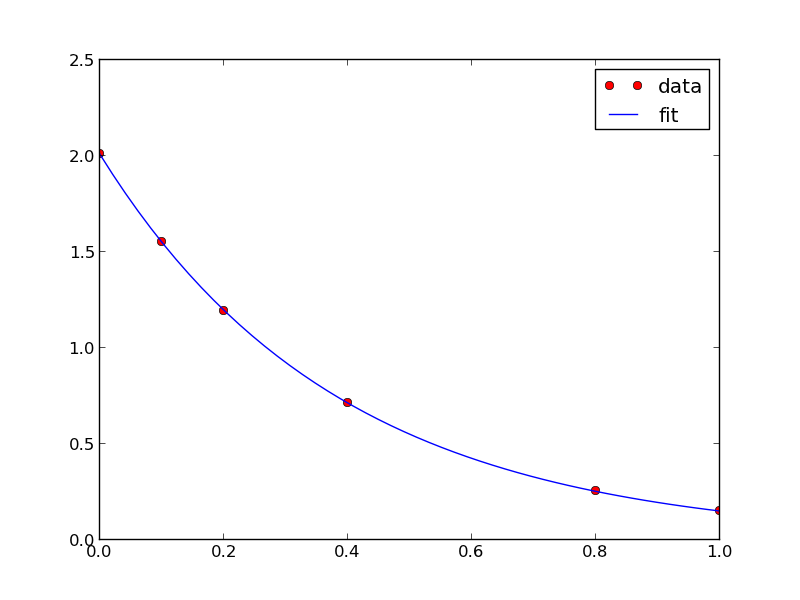
Suppose we know the concentration of A follows this differential equation: \(\frac{dC_A}{dt} = -k C_A\), and we have data we want to fit to it. Here is an example of doing that.

import numpy as np
from scipy.optimize import curve_fit
from scipy.integrate import odeint

# given data we want to fit
tspan = [0, 0.1, 0.2, 0.4, 0.8, 1]
Ca_data = [2.0081,  1.5512,  1.1903,  0.7160,  0.2562,  0.1495]

def fitfunc(t, k):
    'Function that returns Ca computed from an ODE for a k'
    def myode(Ca, t):
        return -k * Ca

    Ca0 = Ca_data[0]
    Casol = odeint(myode, Ca0, t)
    return Casol[:,0]

k_fit, kcov = curve_fit(fitfunc, tspan, Ca_data, p0=1.3)
print k_fit

tfit = np.linspace(0,1);
fit = fitfunc(tfit, k_fit)

import matplotlib.pyplot as plt
plt.plot(tspan, Ca_data, 'ro', label='data')
plt.plot(tfit, fit, 'b-', label='fit')
plt.legend(loc='best')
plt.savefig('images/ode-fit.png')

[ 2.58893455]

org-mode source

Nonlinear curve fitting

Posted February 18, 2013 at 09:00 AM | categories: nonlinear regression, data analysis | tags:

Updated February 27, 2013 at 02:40 PM

Here is a typical nonlinear function fit to data. you need to provide an initial guess. In this example we fit the Birch-Murnaghan equation of state to energy vs. volume data from density functional theory calculations.

from scipy.optimize import leastsq
import numpy as np

vols = np.array([13.71, 14.82, 16.0, 17.23, 18.52])

energies = np.array([-56.29, -56.41, -56.46, -56.463, -56.41])

def Murnaghan(parameters, vol):
    'From Phys. Rev. B 28, 5480 (1983)'
    E0, B0, BP, V0 = parameters

    E = E0 + B0 * vol / BP * (((V0 / vol)**BP) / (BP - 1) + 1) - V0 * B0 / (BP - 1.0)

    return E

def objective(pars, y, x):
    #we will minimize this function
    err =  y - Murnaghan(pars, x)
    return err

x0 = [ -56.0, 0.54, 2.0, 16.5] #initial guess of parameters

plsq = leastsq(objective, x0, args=(energies, vols))

print 'Fitted parameters = {0}'.format(plsq[0])

import matplotlib.pyplot as plt
plt.plot(vols,energies, 'ro')

#plot the fitted curve on top
x = np.linspace(min(vols), max(vols), 50)
y = Murnaghan(plsq[0], x)
plt.plot(x, y, 'k-')
plt.xlabel('Volume')
plt.ylabel('Energy')
plt.savefig('images/nonlinear-curve-fitting.png')

Fitted parameters = [-56.46839641   0.57233217   2.7407944   16.55905648]

See additional examples at \url{http://docs.scipy.org/doc/scipy/reference/tutorial/optimize.html}.

org-mode source