Nonlinear curve fitting
Posted February 18, 2013 at 09:00 AM | categories: data analysis, nonlinear regression | tags:
Updated February 27, 2013 at 02:40 PM
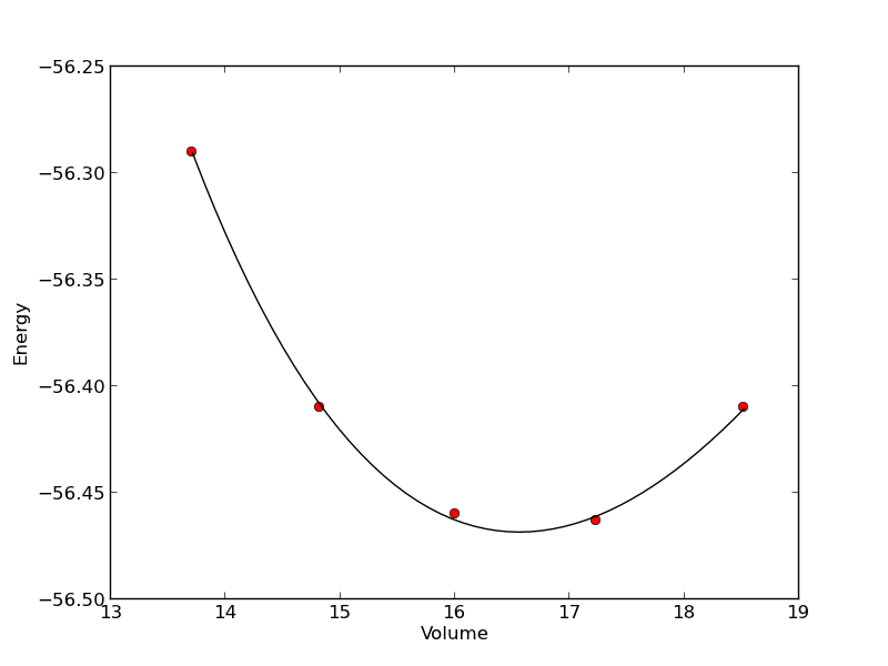
Here is a typical nonlinear function fit to data. you need to provide an initial guess. In this example we fit the Birch-Murnaghan equation of state to energy vs. volume data from density functional theory calculations.
from scipy.optimize import leastsq
import numpy as np

vols = np.array([13.71, 14.82, 16.0, 17.23, 18.52])

energies = np.array([-56.29, -56.41, -56.46, -56.463, -56.41])

def Murnaghan(parameters, vol):
    'From Phys. Rev. B 28, 5480 (1983)'
    E0, B0, BP, V0 = parameters

    E = E0 + B0 * vol / BP * (((V0 / vol)**BP) / (BP - 1) + 1) - V0 * B0 / (BP - 1.0)

    return E

def objective(pars, y, x):
    #we will minimize this function
    err =  y - Murnaghan(pars, x)
    return err

x0 = [ -56.0, 0.54, 2.0, 16.5] #initial guess of parameters

plsq = leastsq(objective, x0, args=(energies, vols))

print 'Fitted parameters = {0}'.format(plsq[0])

import matplotlib.pyplot as plt
plt.plot(vols,energies, 'ro')

#plot the fitted curve on top
x = np.linspace(min(vols), max(vols), 50)
y = Murnaghan(plsq[0], x)
plt.plot(x, y, 'k-')
plt.xlabel('Volume')
plt.ylabel('Energy')
plt.savefig('images/nonlinear-curve-fitting.png')
Fitted parameters = [-56.46839641 0.57233217 2.7407944 16.55905648]
See additional examples at \url{http://docs.scipy.org/doc/scipy/reference/tutorial/optimize.html}.
Copyright (C) 2013 by John Kitchin. See the License for information about copying.