Boundary value problem in heat conduction

| categories: bvp | tags: heat transfer

Matlab post

For steady state heat conduction the temperature distribution in one-dimension is governed by the Laplace equation:

$$ \nabla^2 T = 0$$

with boundary conditions that at \(T(x=a) = T_A\) and \(T(x=L) = T_B\).

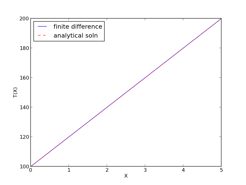
The analytical solution is not difficult here: \(T = T_A-\frac{T_A-T_B}{L}x\), but we will solve this by finite differences.

For this problem, lets consider a slab that is defined by x=0 to x=L, with \(T(x=0) = 100\), and \(T(x=L) = 200\). We want to find the function T(x) inside the slab.

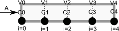
We approximate the second derivative by finite differences as

\( f''(x) \approx \frac{f(x-h) - 2 f(x) + f(x+h)}{h^2} \)

Since the second derivative in this case is equal to zero, we have at each discretized node \(0 = T_{i-1} - 2 T_i + T_{i+1}\). We know the values of \(T_{x=0} = \alpha\) and \(T_{x=L} = \beta\).

\[A = \left [ \begin{array}{ccccc} % -2 & 1 & 0 & 0 & 0 \\ 1 & -2& 1 & 0 & 0 \\ 0 & \ddots & \ddots & \ddots & 0 \\ 0 & 0 & 1 & -2 & 1 \\ 0 & 0 & 0 & 1 & -2 \end{array} \right ] \]

\[ x = \left [ \begin{array}{c} T_1 \\ \vdots \\ T_N \end{array} \right ] \]

\[ b = \left [ \begin{array}{c} -T(x=0) \\ 0 \\ \vdots \\ 0 \\ -T(x=L) \end{array} \right] \]

These are linear equations in the unknowns \(x\) that we can easily solve. Here, we evaluate the solution.

import numpy as np

#we use the notation T(x1) = alpha and T(x2) = beta
x1 = 0; alpha = 100
x2 = 5; beta = 200

npoints = 100

# preallocate and shape the b vector and A-matrix
b = np.zeros((npoints, 1));
b[0] = -alpha
b[-1] = -beta

A = np.zeros((npoints, npoints));

#now we populate the A-matrix and b vector elements
for i in range(npoints ):
    for j in range(npoints):
        if j == i: # the diagonal
            A[i,j] = -2
        elif j == i - 1: # left of the diagonal
            A[i,j] = 1
        elif j == i + 1: # right of the diagonal
            A[i,j] = 1
 
# solve the equations A*y = b for Y
Y = np.linalg.solve(A,b)

x = np.linspace(x1, x2, npoints + 2)
y = np.hstack([alpha, Y[:,0], beta])

import matplotlib.pyplot as plt

plt.plot(x, y)

plt.plot(x, alpha + (beta - alpha)/(x2 - x1) * x, 'r--')

plt.xlabel('X')
plt.ylabel('T(X)')
plt.legend(('finite difference', 'analytical soln'), loc='best')
plt.savefig('images/bvp-heat-conduction-1d.png')

Copyright (C) 2013 by John Kitchin. See the License for information about copying.

org-mode source

Discuss on Twitter

Modeling a transient plug flow reactor

| categories: animation, pde | tags: reaction engineering

Matlab post

The PDE that describes the transient behavior of a plug flow reactor with constant volumetric flow rate is:

\( \frac{\partial C_A}{\partial dt} = -\nu_0 \frac{\partial C_A}{\partial dV} + r_A \).

To solve this numerically in python, we will utilize the method of lines. The idea is to discretize the reactor in volume, and approximate the spatial derivatives by finite differences. Then we will have a set of coupled ordinary differential equations that can be solved in the usual way. Let us simplify the notation with \(C = C_A\), and let \(r_A = -k C^2\). Graphically this looks like this:

This leads to the following set of equations:

\begin{eqnarray} \frac{dC_0}{dt} &=& 0 \text{ (entrance concentration never changes)} \\ \frac{dC_1}{dt} &=& -\nu_0 \frac{C_1 - C_0}{V_1 - V_0} - k C_1^2 \\ \frac{dC_2}{dt} &=& -\nu_0 \frac{C_2 - C_1}{V_2 - V_1} - k C_2^2 \\ \vdots \\ \frac{dC_4}{dt} &=& -\nu_0 \frac{C_4 - C_3}{V_4 - V_3} - k C_4^2 \end{eqnarray}

Last, we need initial conditions for all the nodes in the discretization. Let us assume the reactor was full of empty solvent, so that \(C_i = 0\) at \(t=0\). In the next block of code, we get the transient solutions, and the steady state solution.

import numpy as np
from scipy.integrate import odeint

Ca0 = 2     # Entering concentration
vo = 2      # volumetric flow rate
volume = 20 # total volume of reactor, spacetime = 10
k = 1       # reaction rate constant

N = 100     # number of points to discretize the reactor volume on

init = np.zeros(N)    # Concentration in reactor at t = 0
init[0] = Ca0         # concentration at entrance

V = np.linspace(0, volume, N) # discretized volume elements
tspan = np.linspace(0, 25)    # time span to integrate over

def method_of_lines(C, t):
    'coupled ODES at each node point'
    D = -vo * np.diff(C) / np.diff(V) - k * C[1:]**2
    return np.concatenate([[0], #C0 is constant at entrance
                            D])


sol = odeint(method_of_lines, init, tspan)

# steady state solution
def pfr(C, V):
    return 1.0 / vo * (-k * C**2)

ssol = odeint(pfr, Ca0, V)

The transient solution contains the time dependent behavior of each node in the discretized reactor. Each row contains the concentration as a function of volume at a specific time point. For example, we can plot the concentration of A at the exit vs. time (that is, the last entry of each row) as:

import matplotlib.pyplot as plt
plt.plot(tspan, sol[:, -1])
plt.xlabel('time')
plt.ylabel('$C_A$ at exit')
plt.savefig('images/transient-pfr-1.png')
[<matplotlib.lines.Line2D object at 0x05A18830>]
<matplotlib.text.Text object at 0x059FE1D0>
<matplotlib.text.Text object at 0x05A05270>

After approximately one space time, the steady state solution is reached at the exit. For completeness, we also examine the steady state solution.

plt.figure()
plt.plot(V, ssol, label='Steady state')
plt.plot(V, sol[-1], label='t = {}'.format(tspan[-1]))
plt.xlabel('Volume')
plt.ylabel('$C_A$')
plt.legend(loc='best')
plt.savefig('images/transient-pfr-2.png')

There is some minor disagreement between the final transient solution and the steady state solution. That is due to the approximation in discretizing the reactor volume. In this example we used 100 nodes. You get better agreement with a larger number of nodes, say 200 or more. Of course, it takes slightly longer to compute then, since the number of coupled odes is equal to the number of nodes.

We can also create an animated gif to show how the concentration of A throughout the reactor varies with time. Note, I had to install ffmpeg (http://ffmpeg.org/) to save the animation.

from matplotlib import animation

# make empty figure
fig = plt.figure()
ax = plt.axes(xlim=(0, 20), ylim=(0, 2))
line, = ax.plot(V, init, lw=2)

def animate(i):
    line.set_xdata(V)
    line.set_ydata(sol[i])
    ax.set_title('t = {0}'.format(tspan[i]))
    ax.figure.canvas.draw() 
    return line,
    

anim = animation.FuncAnimation(fig, animate, frames=50,  blit=True)

anim.save('images/transient_pfr.mp4', fps=10)

http://jkitchin.github.com/media/transient_pfr.mp4

You can see from the animation that after about 10 time units, the solution is not changing further, suggesting steady state has been reached.

Copyright (C) 2013 by John Kitchin. See the License for information about copying.

org-mode source

Discuss on Twitter

Integrating the Fermi distribution to compute entropy

| categories: gotcha, integration, dft | tags:

The Fermi distribution is defined by \(f(\epsilon) = \frac{1}{e^{(\epsilon - \mu)/(k T)} + 1}\). This function describes the occupation of energy levels at temperatures above absolute zero. We use this function to compute electronic entropy in a metal, which contains an integral of \(\int n(\epsilon) (f \ln f + (1 - f) \ln (1-f)) d\epsilon\), where \(n(\epsilon)\) is the electronic density of states. Here we plot the Fermi distribution function. It shows that well below the Fermi level the states are fully occupied, and well above the Fermi level, they are unoccupied. Near the Fermi level, the states go from occupied to unoccupied smoothly.

import numpy as np
import matplotlib.pyplot as plt

mu = 0
k = 8.6e-5
T = 1000

def f(e):
    return 1.0 / (np.exp((e - mu)/(k*T)) + 1)

espan = np.linspace(-10, 10, 200)
plt.plot(espan, f(espan))
plt.ylim([-0.1, 1.1])
plt.savefig('images/fermi-entropy-integrand-1.png')

Let us consider a simple density of states function, just a parabola. This could represent a s-band for example. We will use this function to explore the integral.

import numpy as np
import matplotlib.pyplot as plt

mu = 0
k = 8.6e-5
T = 1000

def f(e):
    return 1.0 / (np.exp((e - mu)/(k*T)) + 1)

def dos(e):
    d = (np.ones(e.shape) - 0.03 * e**2) 
    return d * (d > 0)
espan = np.linspace(-10, 10)

plt.plot(espan, dos(espan), label='Total dos')
plt.plot(espan, f(espan) * dos(espan), label='Occupied states')
plt.legend(loc='best')
plt.savefig('images/fermi-entropy-integrand-2.png')

Now, we consider the integral to compute the electronic entropy. The entropy is proportional to this integral.

\( \int n(\epsilon) (f \ln f + (1 - f) \ln (1-f)) d\epsilon \)

It looks straightforward to compute, but it turns out there is a wrinkle. Evaluating the integrand leads to nan elements because the ln(0) is -∞.

import numpy as np
mu = 0
k = 8.6e-5
T = 100

def fermi(e):
    return 1.0 / (np.exp((e - mu)/(k*T)) + 1)

espan = np.array([-20, -10, -5, 0.0, 5, 10])
f = fermi(espan)

print f * np.log(f)
print (1 - f) * np.log(1 - f)
[  0.00000000e+000   0.00000000e+000   0.00000000e+000  -3.46573590e-001
  -1.85216532e-250               nan]
[        nan         nan         nan -0.34657359  0.          0.        ]

In this case, these nan elements should be equal to zero (x ln(x) goes to zero as x goes to zero). So, we can just ignore those elements in the integral. Here is how to do that.

import numpy as np
import matplotlib.pyplot as plt

mu = 0
k = 8.6e-5
T = 1000

def fermi(e):
    return 1.0 / (np.exp((e - mu)/(k*T)) + 1)

def dos(e):
    d = (np.ones(e.shape) - 0.03 * e**2) 
    return d * (d > 0)

espan = np.linspace(-20, 10)
f = fermi(espan)
n = dos(espan)

g = n * (f * np.log(f) + (1 - f) * np.log(1 - f))

print np.trapz(espan, g) # nan because of the nan in the g vector
print g

plt.plot(espan, g)
plt.savefig('images/fermi-entropy-integrand-3.png')

# find the elements that are not nan
ind = np.logical_not(np.isnan(g))

# evaluate the integrand for only those points
print np.trapz(espan[ind], g[ind])
nan
[             nan              nan              nan              nan
              nan              nan              nan              nan
              nan              nan              nan              nan
              nan              nan              nan              nan
              nan              nan              nan              nan
              nan              nan              nan              nan
              nan              nan              nan              nan
  -9.75109643e-14  -1.05987106e-10  -1.04640574e-07  -8.76265644e-05
  -4.92684641e-02  -2.91047740e-01  -7.75652579e-04  -1.00962241e-06
  -1.06972936e-09  -1.00527877e-12  -8.36436686e-16  -6.48930917e-19
  -4.37946336e-22  -2.23285389e-25  -1.88578082e-29   0.00000000e+00
   0.00000000e+00   0.00000000e+00   0.00000000e+00   0.00000000e+00
   0.00000000e+00   0.00000000e+00]
0.208886080897

The integrand is pretty well behaved in the figure above. You do not see the full range of the x-axis, because the integrand evaluates to nan for very negative numbers. This causes the trapz function to return nan also. We can solve the problem by only integrating the parts that are not nan. We have to use numpy.logicalnot to get an element-wise array of which elements are not nan. In this example, the integrand is not well sampled, so the area under that curve may not be very accurate.

Copyright (C) 2013 by John Kitchin. See the License for information about copying.

org-mode source

Discuss on Twitter

An index function for strings in emacs-lisp

| categories: emacs-lisp | tags:

I could not find an index function for strings in emacs-lisp. The position function seems to work for numbers, but not strings. Here is a version that works on strings.

(defun index (item list)
  "return index of item in list or nil"
  (let ((counter 0)
        (found nil))
    (dolist (listelement list counter)
      (if (string= item listelement)
        (progn 
          (setq found t)
          (return counter)) ; exit the loop
        ;; else increment counter
        (incf counter)))
    ;; if we found it return counter otherwise return nil
    (if found counter nil)))
index

Here are some example uses:

(index "test" '("a" "test" "y"))
1
(index "z" '("a" "b" "z"))
2
(index "testy" '("a" "test" "y"))
nil

This raises an error because we use string=.

(index 1 '("a" "test" "y" 1))

Copyright (C) 2013 by John Kitchin. See the License for information about copying.

org-mode source

Discuss on Twitter

Finding the nth root of a periodic function

| categories: nonlinear algebra | tags: heat transfer

There is a heat transfer problem where one needs to find the n^th root of the following equation: \(x J_1(x) - Bi J_0(x)=0\) where \(J_0\) and \(J_1\) are the Bessel functions of zero and first order, and \(Bi\) is the Biot number. We examine an approach to finding these roots.

First, we plot the function.

from scipy.special import jn, jn_zeros
import matplotlib.pyplot as plt
import numpy as np

Bi = 1

def f(x):
    return x * jn(1, x) - Bi * jn(0, x)

X = np.linspace(0, 30, 200)
plt.plot(X, f(X))
plt.savefig('images/heat-transfer-roots-1.png')

You can see there are many roots to this equation, and we want to be sure we get the n^{th} root. This function is pretty well behaved, so if you make a good guess about the solution you will get an answer, but if you make a bad guess, you may get the wrong root. We examine next a way to do it without guessing the solution. What we want is the solution to \(f(x) = 0\), but we want all the solutions in a given interval. We derive a new equation, \(f'(x) = 0\), with initial condition \(f(0) = f0\), and integrate the ODE with an event function that identifies all zeros of \(f\) for us. The derivative of our function is \(df/dx = d/dx(x J_1(x)) - Bi J'_0(x)\). It is known (http://www.markrobrien.com/besselfunct.pdf) that \(d/dx(x J_1(x)) = x J_0(x)\), and \(J'_0(x) = -J_1(x)\). All we have to do now is set up the problem and run it.

from pycse import *  # contains the ode integrator with events

from scipy.special import jn, jn_zeros
import matplotlib.pyplot as plt
import numpy as np

Bi = 1

def f(x):
    "function we want roots for"
    return x * jn(1, x) - Bi * jn(0, x)

def fprime(f, x):
    "df/dx"
    return x * jn(0, x) - Bi * (-jn(1, x))

def e1(f, x):
    "event function to find zeros of f"
    isterminal = False
    value = f
    direction = 0
    return value, isterminal, direction

f0 = f(0)
xspan = np.linspace(0, 30, 200)

x, fsol, XE, FE, IE = odelay(fprime, f0, xspan, events=[e1])

plt.plot(x, fsol, '.-', label='Numerical solution')
plt.plot(xspan, f(xspan), '--', label='Analytical function')
plt.plot(XE, FE, 'ro', label='roots')
plt.legend(loc='best')
plt.savefig('images/heat-transfer-roots-2.png')

for i, root in enumerate(XE):
    print 'root {0} is at {1}'.format(i, root)

plt.show()
root 0 is at 1.25578377377
root 1 is at 4.07947743741
root 2 is at 7.15579904465
root 3 is at 10.2709851256
root 4 is at 13.3983973869
root 5 is at 16.5311587137
root 6 is at 19.6667276775
root 7 is at 22.8039503455
root 8 is at 25.9422288192
root 9 is at 29.081221492

You can work this out once, and then you have all the roots in the interval and you can select the one you want.

Copyright (C) 2013 by John Kitchin. See the License for information about copying.

org-mode source

Discuss on Twitter
« Previous Page -- Next Page »