Some basic data structures in python

| categories: python | tags:

Matlab post

We often have a need to organize data into structures when solving problems.

1 the list

A list in python is data separated by commas in square brackets. Here, we might store the following data in a variable to describe the Antoine coefficients for benzene and the range they are relevant for [Tmin Tmax]. Lists are flexible, you can put anything in them, including other lists. We access the elements of the list by indexing:

c = ['benzene', 6.9056, 1211.0, 220.79, [-16, 104]]
print c[0]
print c[-1]

a,b = c[0:2]
print a,b

name, A, B, C, Trange = c
print Trange
benzene
[-16, 104]
benzene 6.9056
[-16, 104]

Lists are “mutable”, which means you can change their values.

a = [3, 4, 5, [7, 8], 'cat']
print a[0], a[-1]
a[-1] = 'dog'
print a
3 cat
>>> [3, 4, 5, [7, 8], 'dog']

2 tuples

Tuples are immutable; you cannot change their values. This is handy in cases where it is an error to change the value. A tuple is like a list but it is enclosed in parentheses.

a = (3, 4, 5, [7, 8], 'cat')
print a[0], a[-1]
a[-1] = 'dog'
3 cat
Traceback (most recent call last):
  File "<stdin>", line 1, in <module>
TypeError: 'tuple' object does not support item assignment

3 struct

Python does not exactly have the same thing as a struct in Matlab. You can achieve something like it by defining an empty class and then defining attributes of the class. You can check if an object has a particular attribute using hasattr.

class Antoine:
    pass

a = Antoine()
a.name = 'benzene'
a.Trange = [-16, 104]

print a.name
print hasattr(a, 'Trange')
print hasattr(a, 'A')
benzene
True
False

4 dictionaries

The analog of the containers.Map in Matlab is the dictionary in python. Dictionaries are enclosed in curly brackets, and are composed of key:value pairs.

s = {'name':'benzene',
     'A':6.9056,
     'B':1211.0}

s['C'] = 220.79
s['Trange'] = [-16, 104]

print s
print s['Trange']
{'A': 6.9056, 'C': 220.79, 'B': 1211.0, 'name': 'benzene', 'Trange': [-16, 104]}
[-16, 104]
s = {'name':'benzene',
     'A':6.9056,
     'B':1211.0}

print 'C' in s
# default value for keys not in the dictionary
print s.get('C', None)

print s.keys()
print s.values()
False
None
['A', 'B', 'name']
[6.9056, 1211.0, 'benzene']

5 Summary

We have examined four data structures in python. Note that none of these types are arrays/vectors with defined mathematical operations. For those, you need to consider numpy.array.

Copyright (C) 2013 by John Kitchin. See the License for information about copying.
org-mode source

Discuss on Twitter

Creating arrays in python

| categories: python | tags:

Often, we will have a set of 1-D arrays, and we would like to construct a 2D array with those vectors as either the rows or columns of the array. This may happen because we have data from different sources we want to combine, or because we organize the code with variables that are easy to read, and then want to combine the variables. Here are examples of doing that to get the vectors as the columns.

import numpy as np

a = np.array([1, 2, 3])
b = np.array([4, 5, 6])

print np.column_stack([a, b])

# this means stack the arrays vertically, e.g. on top of each other
print np.vstack([a, b]).T
[[1 4]
 [2 5]
 [3 6]]
[[1 4]
 [2 5]
 [3 6]]

Or rows:

import numpy as np

a = np.array([1, 2, 3])
b = np.array([4, 5, 6])

print np.row_stack([a, b])

# this means stack the arrays vertically, e.g. on top of each other
print np.vstack([a, b])
[[1 2 3]
 [4 5 6]]
[[1 2 3]
 [4 5 6]]

The opposite operation is to extract the rows or columns of a 2D array into smaller arrays. We might want to do that to extract a row or column from a calculation for further analysis, or plotting for example. There are splitting functions in numpy. They are somewhat confusing, so we examine some examples. The numpy.hsplit command splits an array “horizontally”. The best way to think about it is that the “splits” move horizontally across the array. In other words, you draw a vertical split, move over horizontally, draw another vertical split, etc… You must specify the number of splits that you want, and the array must be evenly divisible by the number of splits.

import numpy as np

A = np.array([[1, 2, 3, 5], 
              [4, 5, 6, 9]])

# split into two parts
p1, p2 = np.hsplit(A, 2)
print p1
print p2

#split into 4 parts
p1, p2, p3, p4 = np.hsplit(A, 4)
print p1
print p2
print p3
print p4
[[1 2]
 [4 5]]
[[3 5]
 [6 9]]
[[1]
 [4]]
[[2]
 [5]]
[[3]
 [6]]
[[5]
 [9]]

In the numpy.vsplit command the “splits” go “vertically” down the array. Note that the split commands return 2D arrays.

import numpy as np

A = np.array([[1, 2, 3, 5], 
              [4, 5, 6, 9]])

# split into two parts
p1, p2 = np.vsplit(A, 2)
print p1
print p2
print p2.shape
[[1 2 3 5]]
[[4 5 6 9]]
(1, 4)

An alternative approach is array unpacking. In this example, we unpack the array into two variables. The array unpacks by row.

import numpy as np

A = np.array([[1, 2, 3, 5], 
              [4, 5, 6, 9]])

# split into two parts
p1, p2 = A
print p1
print p2
[1 2 3 5]
[4 5 6 9]

To get the columns, just transpose the array.

import numpy as np

A = np.array([[1, 2, 3, 5], 
              [4, 5, 6, 9]])

# split into two parts
p1, p2, p3, p4 = A.T
print p1
print p2
print p3
print p4
print p4.shape
[1 4]
[2 5]
[3 6]
[5 9]
(2,)

Note that now, we have 1D arrays.

You can also access rows and columns by indexing. We index an array by [row, column]. To get a row, we specify the row number, and all the columns in that row like this [row, :]. Similarly, to get a column, we specify that we want all rows in that column like this: [:, column]. This approach is useful when you only want a few columns or rows.

import numpy as np

A = np.array([[1, 2, 3, 5], 
              [4, 5, 6, 9]])

# get row 1
print A[1]
print A[1, :]  # row 1, all columns

print A[:, 2]  # get third column 
print A[:, 2].shape
[4 5 6 9]
[4 5 6 9]
[3 6]
(2,)

Note that even when we specify a column, it is returned as a 1D array.

Copyright (C) 2013 by John Kitchin. See the License for information about copying.

org-mode source

Discuss on Twitter

Advanced string formatting

| categories: python | tags:

There are several more advanced ways to include formatted values in a string. In the previous case we examined replacing format specifiers by positional arguments in the format command. We can instead use keyword arguments.

s = 'The {speed} {color} fox'.format(color='brown', speed='quick')
print s
The quick brown fox

If you have a lot of variables already defined in a script, it is convenient to use them in string formatting with the locals command:

speed = 'slow'
color= 'blue'

print 'The {speed} {color} fox'.format(**locals())
The slow blue fox

If you want to access attributes on an object, you can specify them directly in the format identifier.

class A:
    def __init__(self, a, b, c):
        self.a = a
        self.b = b
        self.c = c

mya = A(3,4,5)

print 'a = {obj.a}, b = {obj.b}, c = {obj.c:1.2f}'.format(obj=mya)
a = 3, b = 4, c = 5.00

You can access values of a dictionary:

d = {'a': 56, "test":'woohoo!'}

print "the value of a in the dictionary is {obj[a]}. It works {obj[test]}".format(obj=d)
the value of a in the dictionary is 56. It works woohoo!.

And, you can access elements of a list. Note, however you cannot use -1 as an index in this case.

L = [4, 5, 'cat']

print 'element 0 = {obj[0]}, and the last element is {obj[2]}'.format(obj=L)
element 0 = 4, and the last element is cat

There are three different ways to “print” an object. If an object has a format function, that is the default used in the format command. It may be helpful to use the str or repr of an object instead. We get this with !s for str and !r for repr.

class A:
    def __init__(self, a, b):
        self.a = a; self.b = b

    def __format__(self, format):
        s = 'a={{0:{0}}} b={{1:{0}}}'.format(format)
        return s.format(self.a, self.b)

    def __str__(self):
        return 'str: class A, a={0} b={1}'.format(self.a, self.b)

    def __repr__(self):
        return 'representing: class A, a={0}, b={1}'.format(self.a, self.b)

mya = A(3, 4)

print '{0}'.format(mya)   # uses __format__
print '{0!s}'.format(mya) # uses __str__
print '{0!r}'.format(mya) # uses __repr__
a=3 b=4
str: class A, a=3 b=4
representing: class A, a=3, b=4

This covers the majority of string formatting requirements I have come across. If there are more sophisticated needs, they can be met with various string templating python modules. the one I have used most is Cheetah.

Copyright (C) 2013 by John Kitchin. See the License for information about copying.

org-mode source

Discuss on Twitter

Integrating functions in python

| categories: math, python | tags:

Matlab post

Problem statement

find the integral of a function f(x) from a to b i.e.

$$\int_a^b f(x) dx$$

In python we use numerical quadrature to achieve this with the scipy.integrate.quad command.

as a specific example, lets integrate

$$y=x^2$$

from x=0 to x=1. You should be able to work out that the answer is 1/3.

from scipy.integrate import quad

def integrand(x):
    return x**2

ans, err = quad(integrand, 0, 1)
print ans
0.333333333333

1 double integrals

we use the scipy.integrate.dblquad command

Integrate \(f(x,y)=y sin(x)+x cos(y)\) over

\(\pi <= x <= 2\pi\)

\(0 <= y <= \pi\)

i.e.

\(\int_{x=\pi}^{2\pi}\int_{y=0}^{\pi}y sin(x)+x cos(y)dydx\)

The syntax in dblquad is a bit more complicated than in Matlab. We have to provide callable functions for the range of the y-variable. Here they are constants, so we create lambda functions that return the constants. Also, note that the order of arguments in the integrand is different than in Matlab.

from scipy.integrate import dblquad
import numpy as np

def integrand(y, x):
    'y must be the first argument, and x the second.'
    return y * np.sin(x) + x * np.cos(y)

ans, err = dblquad(integrand, np.pi, 2*np.pi,
                   lambda x: 0,
                   lambda x: np.pi)
print ans
-9.86960440109

we use the tplquad command to integrate \(f(x,y,z)=y sin(x)+z cos(x)\) over the region

\(0 <= x <= \pi\)

\(0 <= y <= 1\)

\(-1 <= z <= 1\)

from scipy.integrate import tplquad
import numpy as np

def integrand(z, y, x):
    return y * np.sin(x) + z * np.cos(x)

ans, err = tplquad(integrand,
                   0, np.pi,  # x limits
                   lambda x: 0,
                   lambda x: 1, # y limits
                   lambda x,y: -1,
                   lambda x,y: 1) # z limits

print ans
2.0

2 Summary

scipy.integrate offers the same basic functionality as Matlab does. The syntax differs significantly for these simple examples, but the use of functions for the limits enables freedom to integrate over non-constant limits.

Copyright (C) 2013 by John Kitchin. See the License for information about copying.

org-mode source

Discuss on Twitter

On the quad or trapz'd in ChemE heaven

| categories: integration, python | tags:

Matlab post

What is the difference between quad and trapz? The short answer is that quad integrates functions (via a function handle) using numerical quadrature, and trapz performs integration of arrays of data using the trapezoid method.

Let us look at some examples. We consider the example of computing \(\int_0^2 x^3 dx\). the analytical integral is \(1/4 x^4\), so we know the integral evaluates to 16/4 = 4. This will be our benchmark for comparison to the numerical methods.

We use the scipy.integrate.quad command to evaluate this \(\int_0^2 x^3 dx\).

from scipy.integrate import quad

ans, err = quad(lambda x: x**3, 0, 2)
print ans
4.0

you can also define a function for the integrand.

from scipy.integrate import quad

def integrand(x):
    return x**3

ans, err = quad(integrand, 0, 2)
print ans
4.0

1 Numerical data integration

if we had numerical data like this, we use trapz to integrate it

import numpy as np

x = np.array([0, 0.5, 1, 1.5, 2])
y = x**3

i2 = np.trapz(y, x)

error = (i2 - 4)/4

print i2, error
4.25 0.0625

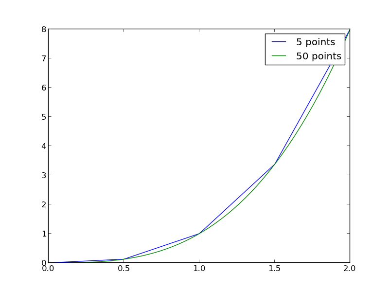
Note the integral of these vectors is greater than 4! You can see why here.

import numpy as np
import matplotlib.pyplot as plt
x = np.array([0, 0.5, 1, 1.5, 2])
y = x**3

x2 = np.linspace(0, 2)
y2 = x2**3

plt.plot(x, y, label='5 points')
plt.plot(x2, y2, label='50 points')
plt.legend()
plt.savefig('images/quad-1.png')

The trapezoid method is overestimating the area significantly. With more points, we get much closer to the analytical value.

import numpy as np

x2 = np.linspace(0, 2, 100)
y2 = x2**3

print np.trapz(y2, x2)
4.00040812162

2 Combining numerical data with quad

You might want to combine numerical data with the quad function if you want to perform integrals easily. Let us say you are given this data:

x = [0 0.5 1 1.5 2]; y = [0 0.1250 1.0000 3.3750 8.0000];

and you want to integrate this from x = 0.25 to 1.75. We do not have data in those regions, so some interpolation is going to be needed. Here is one approach.

from scipy.interpolate import interp1d
from scipy.integrate import quad
import numpy as np

x = [0, 0.5, 1, 1.5, 2]
y = [0,    0.1250,    1.0000,    3.3750,    8.0000]

f = interp1d(x, y)

# numerical trapezoid method
xfine = np.linspace(0.25, 1.75)
yfine = f(xfine)
print np.trapz(yfine, xfine)

# quadrature with interpolation
ans, err = quad(f, 0.25, 1.75)
print ans
2.53199187838
2.53125

These approaches are very similar, and both rely on linear interpolation. The second approach is simpler, and uses fewer lines of code.

3 Summary

trapz and quad are functions for getting integrals. Both can be used with numerical data if interpolation is used. The syntax for the quad and trapz function is different in scipy than in Matlab.

Finally, see this post for an example of solving an integral equation using quad and fsolve.

Copyright (C) 2013 by John Kitchin. See the License for information about copying.

org-mode source

Discuss on Twitter
« Previous Page -- Next Page »