A new ode integrator function in scipy

| categories: ode, scipy | tags:

I learned recently about a new way to solve ODEs in scipy: scipy.integrate.solve_ivp. This new function is recommended instead of scipy.integrate.odeint for new code. This function caught my eye because it added functionality that was previously missing, and that I had written into my pycse package. That functionality is events.

To explore how to use this new function, I will recreate an old blog post where I used events to count the number of roots in a function. Spoiler alert: it may not be ready for production.

The question at hand is how many roots are there in \(f(x) = x^3 + 6x^2 - 4x - 24\), and what are they. Now, I know there are three roots and that you can use np.roots for this, but that only works for polynomials. Here they are, so we know what we are looking for.

import numpy as np
np.roots([1, 6, -4, -24])
array([-6.,  2., -2.])

The point of this is to find a more general way to count roots in an interval. We do it by integrating the derivative of the function, and using an event function to count when the function is equal to zero. First, we define the derivative:

\(f'(x) = 3x^2 + 12x - 4\), and the value of our original function at some value that is the beginning of the range we want to consider, say \(f(-8) = -120\). Now, we have an ordinary differential equation that can be integrated. Our event function is simply, it is just the function value \(y\). In the next block, I include an optional t_eval arg so we can see the solution at more points.

def fprime(x, y):
    return 3 * x**2 + 12 * x - 4

def event(x, y):
    return y

import numpy as np
from scipy.integrate import solve_ivp
sol = solve_ivp(fprime, (-8, 4), np.array([-120]), t_eval=np.linspace(-8, 4, 10), events=[event])
sol
 message: 'The solver successfully reached the interval end.'
    nfev: 26
    njev: 0
     nlu: 0
     sol: None
  status: 0
 success: True
       t: array([-8.        , -6.66666667, -5.33333333, -4.        , -2.66666667,
      -1.33333333,  0.        ,  1.33333333,  2.66666667,  4.        ])
t_events: [array([-6.])]
       y: array([[-120.        ,  -26.96296296,   16.2962963 ,   24.        ,
         10.37037037,  -10.37037037,  -24.        ,  -16.2962963 ,
         26.96296296,  120.        ]])

sol.t_events
[array([-6.])]

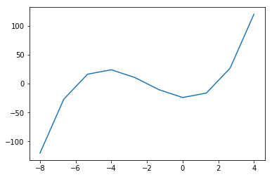
Huh. That is not what I expected. There should be three values in sol.t_events, but there is only one. Looking at sol.y, you can see there are three sign changes, which means three zeros. The graph here confirms that.

%matplotlib inline
import matplotlib.pyplot as plt
plt.plot(sol.t, sol.y[0])
[<matplotlib.lines.Line2D at 0x151281d860>]

What appears to be happening is that the events are only called during the solver steps, which are different than the t_eval steps. It appears a workaround is to specify a max_step that can be taken by the solver to force the event functions to be evaluated more often. Adding this seems to create a new cryptic warning.

sol = solve_ivp(fprime, (-8, 4), np.array([-120]), events=[event], max_step=1.0)
sol
/Users/jkitchin/anaconda/lib/python3.6/site-packages/scipy/integrate/_ivp/rk.py:145: RuntimeWarning: divide by zero encountered in double_scalars
  max(1, SAFETY * error_norm ** (-1 / (order + 1))))


 message: 'The solver successfully reached the interval end.'
    nfev: 80
    njev: 0
     nlu: 0
     sol: None
  status: 0
 success: True
       t: array([-8.        , -7.89454203, -6.89454203, -5.89454203, -4.89454203,
      -3.89454203, -2.89454203, -1.89454203, -0.89454203,  0.10545797,
       1.10545797,  2.10545797,  3.10545797,  4.        ])
t_events: [array([-6., -2.,  2.])]
       y: array([[-120.        , -110.49687882,  -38.94362768,    3.24237128,
         22.06111806,   23.51261266,   13.59685508,   -1.68615468,
        -16.33641662,  -24.35393074,  -19.73869704,    3.50928448,
         51.39001383,  120.        ]])

sol.t_events
[array([-6., -2.,  2.])]

That is more like it. Here, I happen to know the answers, so we are safe setting a max_step of 1.0, but that feels awkward and unreliable. You don't want this max_step to be too small, because it probably makes for more computations. On the other hand, it can't be too large either because you might miss roots. It seems there is room for improvement on this.

It also seems odd that the solve_ivp only returns the t_events, and not also the corresponding solution values. I guess in this case, we know the solution values are zero at t_events, but, supposing you instead were looking for a maximum value by getting a derivative that was equal to zero, you might end up getting stuck solving for it some how.

Let's consider this parabola with a maximum at \(x=2\), where \(y=2\):

x = np.linspace(0, 4)
plt.plot(x, 2 - (x - 2)**2)
[<matplotlib.lines.Line2D at 0x1512dad9e8>]

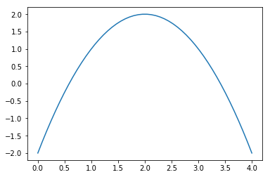
We can find the maximum like this.

def yprime(x, y):
    return -2  * (x - 2)

def maxevent(x, y):
    return yprime(x, y)

sol = solve_ivp(yprime, (0, 4), np.array([-2]), events=[maxevent])
sol
/Users/jkitchin/anaconda/lib/python3.6/site-packages/scipy/integrate/_ivp/rk.py:145: RuntimeWarning: divide by zero encountered in double_scalars
  max(1, SAFETY * error_norm ** (-1 / (order + 1))))


 message: 'The solver successfully reached the interval end.'
    nfev: 20
    njev: 0
     nlu: 0
     sol: None
  status: 0
 success: True
       t: array([ 0.        ,  0.08706376,  0.95770136,  4.        ])
t_events: [array([ 2.])]
       y: array([[-2.        , -1.65932506,  0.91361355, -2.        ]])

Clearly, we found the maximum at x=2, but now what? Re-solve the ODE and use t_eval with the t_events values? Use a fine t_eval array, and interpolate the solution? That doesn't seem smart. You could make the event terminal, so that it stops at the max, and then read off the last value, but this will not work if you want to count more than one maximum, for example.

maxevent.terminal = True
solve_ivp(yprime, (0, 4), (-2,), events=[maxevent])
/Users/jkitchin/anaconda/lib/python3.6/site-packages/scipy/integrate/_ivp/rk.py:145: RuntimeWarning: divide by zero encountered in double_scalars
  max(1, SAFETY * error_norm ** (-1 / (order + 1))))


 message: 'A termination event occurred.'
    nfev: 20
    njev: 0
     nlu: 0
     sol: None
  status: 1
 success: True
       t: array([ 0.        ,  0.08706376,  0.95770136,  2.        ])
t_events: [array([ 2.])]
       y: array([[-2.        , -1.65932506,  0.91361355,  2.        ]])

Internet: am I missing something obvious here?

Copyright (C) 2018 by John Kitchin. See the License for information about copying.

org-mode source

Org-mode version = 9.1.13

Discuss on Twitter

Solving ODEs with a neural network and autograd

| categories: autograd, ode | tags:

In the last post I explored using a neural network to solve a BVP. Here, I expand the idea to solving an initial value ordinary differential equation. The idea is basically the same, we just have a slightly different objective function.

\(dCa/dt = -k Ca(t)\) where \(Ca(t=0) = 2.0\).

Here is the code that solves this equation, along with a comparison to the analytical solution: \(Ca(t) = Ca0 \exp -kt\).

import autograd.numpy as np
from autograd import grad, elementwise_grad
import autograd.numpy.random as npr
from autograd.misc.optimizers import adam

def init_random_params(scale, layer_sizes, rs=npr.RandomState(0)):
    """Build a list of (weights, biases) tuples, one for each layer."""
    return [(rs.randn(insize, outsize) * scale,   # weight matrix
             rs.randn(outsize) * scale)           # bias vector
            for insize, outsize in zip(layer_sizes[:-1], layer_sizes[1:])]


def swish(x):
    "see https://arxiv.org/pdf/1710.05941.pdf"
    return x / (1.0 + np.exp(-x))


def Ca(params, inputs):
    "Neural network functions"
    for W, b in params:
        outputs = np.dot(inputs, W) + b
        inputs = swish(outputs)    
    return outputs

    
# Here is our initial guess of params:
params = init_random_params(0.1, layer_sizes=[1, 8, 1])

# Derivatives
dCadt = elementwise_grad(Ca, 1)

k = 0.23
Ca0 = 2.0
t = np.linspace(0, 10).reshape((-1, 1))

# This is the function we seek to minimize
def objective(params, step):
    # These should all be zero at the solution
    # dCadt = -k * Ca(t)
    zeq = dCadt(params, t) - (-k * Ca(params, t))
    ic = Ca(params, 0) - Ca0
    return np.mean(zeq**2) + ic**2

def callback(params, step, g):
    if step % 1000 == 0:
        print("Iteration {0:3d} objective {1}".format(step,
                                                      objective(params, step)))

params = adam(grad(objective), params,
              step_size=0.001, num_iters=5001, callback=callback) 


tfit = np.linspace(0, 20).reshape(-1, 1)
import matplotlib.pyplot as plt
plt.plot(tfit, Ca(params, tfit), label='soln')
plt.plot(tfit, Ca0 * np.exp(-k * tfit), 'r--', label='analytical soln')
plt.legend()
plt.xlabel('time')
plt.ylabel('$C_A$')
plt.xlim([0, 20])
plt.savefig('nn-ode.png')
Iteration   0 objective [[ 3.20374053]]
Iteration 1000 objective [[  3.13906829e-05]]
Iteration 2000 objective [[  1.95894699e-05]]
Iteration 3000 objective [[  1.60381564e-05]]
Iteration 4000 objective [[  1.39930673e-05]]
Iteration 5000 objective [[  1.03554970e-05]]

Huh. Those two solutions are nearly indistinguishable. Since we used a neural network, let's hype it up and say we learned the solution to a differential equation! But seriously, note that although we got an "analytical" solution, we should only rely on it in the region we trained the solution on. You can see the solution above is not that good past t=10, even perhaps going negative (which is not even physically correct). That is a reminder that the function we have for the solution is not the same as the analytical solution, it just approximates it really well over the region we solved over. Of course, you can expand that region to the region you care about, but the main point is don't rely on the solution outside where you know it is good.

This idea isn't new. There are several papers in the literature on using neural networks to solve differential equations, e.g. http://www.sciencedirect.com/science/article/pii/S0255270102002076 and https://arxiv.org/pdf/physics/9705023.pdf, and other blog posts that are similar (https://becominghuman.ai/neural-networks-for-solving-differential-equations-fa230ac5e04c, even using autograd). That means to me that there is some merit to continuing to investigate this approach to solving differential equations.

There are some interesting challenges for engineers to consider with this approach though. When is the solution accurate enough? How reliable are derivatives of the solution? What network architecture is appropriate or best? How do you know how good the solution is? Is it possible to build in solution features, e.g. asymptotes, or constraints on derivatives, or that the solution should be monotonic, etc. These would help us trust the solutions not to do weird things, and to extrapolate more reliably.

Copyright (C) 2017 by John Kitchin. See the License for information about copying.

org-mode source

Org-mode version = 9.1.2

Discuss on Twitter

Uncertainty in the solution of an ODE

| categories: uncertainty, ode | tags:

Our objective in this post is to examine the effects of uncertainty in parameters that define an ODE on the integrated solution of the ODE. My favorite method for numerical uncertainty analysis is Monte Carlo simulation because it is easy to code and usually easy to understand. We take that approach first.

The problem to solve is to estimate the conversion in a constant volume batch reactor with a second order reaction \(A \rightarrow B\), and the rate law: \(-r_A = k C_A^2\), after one hour of reaction. There is 5% uncertainty in the rate constant \(k=0.001\) and in the initial concentration \(C_{A0}=1\).

The relevant differential equation is:

\(\frac{dX}{dt} = -r_A /C_{A0}\).

We have to assume that 5% uncertainty refers to a normal distribution of error that has a standard deviation of 5% of the mean value.

from scipy.integrate import odeint
import numpy as np

N = 1000

K = np.random.normal(0.001, 0.05*0.001, N)
CA0 = np.random.normal(1, 0.05*1, N)

X = [] # to store answer in
for k, Ca0 in zip(K, CA0):
    # define ODE
    def ode(X, t):
        ra = -k * (Ca0 * (1 - X))**2
        return -ra / Ca0
    
    X0 = 0
    tspan = np.linspace(0,3600)

    sol = odeint(ode, X0, tspan)

    X += [sol[-1][0]]

s = 'Final conversion at one hour is {0:1.3f} +- {1:1.3f} (1 sigma)'
print s.format(np.average(X),
               np.std(X))
Final conversion at one hour is 0.782 +- 0.013 (1 sigma)

See, it is not too difficulty to write. It is however, a little on the expensive side to run, since we typically need 1e3-1e6 samples to get the statistics reasonable. Let us try the uncertainties package too. For this we have to wrap a function that takes uncertainties and returns a single float number.

from scipy.integrate import odeint
import numpy as np
import uncertainties as u

k = u.ufloat(0.001, 0.05*0.001)
Ca0 = u.ufloat(1.0, 0.05)

@u.wrap
def func(k, Ca0):
    # define the ODE
    def ode(X, t):
        ra = -k * (Ca0 * (1 - X))**2
        return -ra / Ca0
    
    X0 = 0 # initial condition
    tspan = np.linspace(0, 3600)
    # integrate it
    sol = odeint(ode, X0, tspan)
    return sol[-1][0]

result = func(k, Ca0)
s = 'Final conversion at one hour is {0}(1 sigma)'
print s.format(result)
Final conversion at one hour is 0.783+/-0.012(1 sigma)

This is about the same amount of code as the Monte Carlo approach, but it runs much faster, and gets approximately the same results. You have to remember the wrapping technique, since the uncertainties package does not run natively with the odeint function.

Copyright (C) 2013 by John Kitchin. See the License for information about copying.

org-mode source

Discuss on Twitter

Linear algebra approaches to solving systems of constant coefficient ODEs

| categories: ode | tags:

Matlab post Today we consider how to solve a system of first order, constant coefficient ordinary differential equations using linear algebra. These equations could be solved numerically, but in this case there are analytical solutions that can be derived. The equations we will solve are:

\(y'_1 = -0.02 y_1 + 0.02 y_2\)

\(y'_2 = 0.02 y_1 - 0.02 y_2\)

We can express this set of equations in matrix form as: \(\left[\begin{array}{c}y'_1\\y'_2\end{array}\right] = \left[\begin{array}{cc} -0.02 & 0.02 \\ 0.02 & -0.02\end{array}\right] \left[\begin{array}{c}y_1\\y_2\end{array}\right]\)

The general solution to this set of equations is

\(\left[\begin{array}{c}y_1\\y_2\end{array}\right] = \left[\begin{array}{cc}v_1 & v_2\end{array}\right] \left[\begin{array}{cc} c_1 & 0 \\ 0 & c_2\end{array}\right] \exp\left(\left[\begin{array}{cc} \lambda_1 & 0 \\ 0 & \lambda_2\end{array}\right] \left[\begin{array}{c}t\\t\end{array}\right]\right)\)

where \(\left[\begin{array}{cc} \lambda_1 & 0 \\ 0 & \lambda_2\end{array}\right]\) is a diagonal matrix of the eigenvalues of the constant coefficient matrix, \(\left[\begin{array}{cc}v_1 & v_2\end{array}\right]\) is a matrix of eigenvectors where the \(i^{th}\) column corresponds to the eigenvector of the \(i^{th}\) eigenvalue, and \(\left[\begin{array}{cc} c_1 & 0 \\ 0 & c_2\end{array}\right]\) is a matrix determined by the initial conditions.

In this example, we evaluate the solution using linear algebra. The initial conditions we will consider are \(y_1(0)=0\) and \(y_2(0)=150\).

import numpy as np

A = np.array([[-0.02,  0.02],
              [ 0.02, -0.02]])

# Return the eigenvalues and eigenvectors of a Hermitian or symmetric matrix.
evals, evecs = np.linalg.eigh(A)
print evals
print evecs
>>> ... >>> >>> ... >>> [-0.04  0.  ]
[[ 0.70710678  0.70710678]
 [-0.70710678  0.70710678]]

The eigenvectors are the columns of evecs.

Compute the \(c\) matrix

V*c = Y0

Y0 = [0, 150]

c = np.diag(np.linalg.solve(evecs, Y0))
print c
>>> >>> [[-106.06601718    0.        ]
 [   0.          106.06601718]]

Constructing the solution

We will create a vector of time values, and stack them for each solution, \(y_1(t)\) and \(Y_2(t)\).

import matplotlib.pyplot as plt

t = np.linspace(0, 100)
T = np.row_stack([t, t])

D = np.diag(evals)

# y = V*c*exp(D*T);
y = np.dot(np.dot(evecs, c), np.exp(np.dot(D, T)))

# y has a shape of (2, 50) so we have to transpose it
plt.plot(t, y.T)
plt.xlabel('t')
plt.ylabel('y')
plt.legend(['$y_1$', '$y_2$'])
plt.savefig('images/ode-la.png')
plt.show()
>>> >>> >>> >>> ... >>> >>> ... [<matplotlib.lines.Line2D object at 0x1d4db950>, <matplotlib.lines.Line2D object at 0x1d4db4d0>]
<matplotlib.text.Text object at 0x1d35fbd0>
<matplotlib.text.Text object at 0x1c222390>
<matplotlib.legend.Legend object at 0x1d34ee90>

Copyright (C) 2013 by John Kitchin. See the License for information about copying.

org-mode source

Discuss on Twitter

Another way to parameterize an ODE - nested function

| categories: ode | tags:

Matlab post We saw one method to parameterize an ODE, by creating an ode function that takes an extra parameter argument, and then making a function handle that has the syntax required for the solver, and passes the parameter the ode function.

Here we define the ODE function in a loop. Since the nested function is in the namespace of the main function, it can “see” the values of the variables in the main function. We will use this method to look at the solution to the van der Pol equation for several different values of mu.

import numpy as np
from scipy.integrate import odeint
import matplotlib.pyplot as plt

MU = [0.1, 1, 2, 5]
tspan = np.linspace(0, 100, 5000)
Y0 = [0, 3]

for mu in MU:
    # define the ODE
    def vdpol(Y, t):
        x,y = Y
        dxdt = y
        dydt = -x + mu * (1 - x**2) * y
        return  [dxdt, dydt]
    
    Y = odeint(vdpol, Y0, tspan)
    
    x = Y[:,0]; y = Y[:,1]
    plt.plot(x, y, label='mu={0:1.2f}'.format(mu))

plt.axis('equal')
plt.legend(loc='best')
plt.savefig('images/ode-nested-parameterization.png')
plt.show()

You can see the solution changes dramatically for different values of mu. The point here is not to understand why, but to show an easy way to study a parameterize ode with a nested function. Nested functions can be a great way to “share” variables between functions especially for ODE solving, and nonlinear algebra solving, or any other application where you need a lot of parameters defined in one function in another function.

Copyright (C) 2013 by John Kitchin. See the License for information about copying.

org-mode source

Discuss on Twitter
« Previous Page -- Next Page »