Yet another way to parameterize an ODE

| categories: ode | tags:

Matlab post We previously examined a way to parameterize an ODE. In those methods, we either used an anonymous function to parameterize an ode function, or we used a nested function that used variables from the shared workspace.

We want a convenient way to solve \(dCa/dt = -k Ca\) for multiple values of \(k\). Here we use a trick to pass a parameter to an ODE through the initial conditions. We expand the ode function definition to include this parameter, and set its derivative to zero, effectively making it a constant.

import numpy as np
from scipy.integrate import odeint
import matplotlib.pyplot as plt

def ode(F, t):
    Ca, k = F
    dCadt = -k * Ca
    dkdt = 0.0
    return [dCadt, dkdt]

tspan = np.linspace(0, 4)

Ca0 = 1;
K = [2.0, 3.0]
for k in K:
    F = odeint(ode, [Ca0, k], tspan)
    Ca = F[:,0]
    plt.plot(tspan, Ca, label='k={0}'.format(k))
plt.xlabel('time')
plt.ylabel('$C_A$')
plt.legend(loc='best')
plt.savefig('images/ode-parameterized-1.png')
plt.show()

I do not think this is a very elegant way to pass parameters around compared to the previous methods, but it nicely illustrates that there is more than one way to do it. And who knows, maybe it will be useful in some other context one day!

Copyright (C) 2013 by John Kitchin. See the License for information about copying.

org-mode source

Discuss on Twitter

Error tolerance in numerical solutions to ODEs

| categories: ode | tags:

Matlab post Usually, the numerical ODE solvers in python work well with the standard settings. Sometimes they do not, and it is not always obvious they have not worked! Part of using a tool like python is checking how well your solution really worked. We use an example of integrating an ODE that defines the van der Waal equation of an ideal gas here.

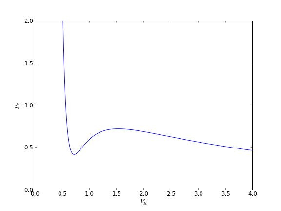
we plot the analytical solution to the van der waal equation in reduced form here.

import numpy as np
import matplotlib.pyplot as plt

Tr = 0.9
Vr = np.linspace(0.34,4,1000)

#analytical equation for Pr
Prfh = lambda Vr: 8.0 / 3.0 * Tr / (Vr - 1.0 / 3.0) - 3.0 / (Vr**2)
Pr = Prfh(Vr) # evaluated on our reduced volume vector.

# Plot the EOS
plt.plot(Vr,Pr)
plt.ylim([0, 2])
plt.xlabel('$V_R$')
plt.ylabel('$P_R$')
plt.savefig('images/ode-vw-1.png')
plt.show()
>>> >>> >>> >>> >>> ... >>> >>> >>> ... [<matplotlib.lines.Line2D object at 0x1c5a3550>]
(0, 2)
<matplotlib.text.Text object at 0x1c22f750>
<matplotlib.text.Text object at 0x1d4e0750>

we want an equation for dPdV, which we will integrate we use symbolic math to do the derivative for us.

from sympy import diff, Symbol
Vrs = Symbol('Vrs')

Prs = 8.0 / 3.0 * Tr / (Vrs - 1.0/3.0) - 3.0/(Vrs**2) 
print diff(Prs,Vrs)
>>> -2.4/(Vrs - 0.333333333333333)**2 + 6.0/Vrs**3

Now, we solve the ODE. We will specify a large relative tolerance criteria (Note the default is much smaller than what we show here).

from scipy.integrate import odeint

def myode(Pr, Vr):
    dPrdVr = -2.4/(Vr - 0.333333333333333)**2 + 6.0/Vr**3
    return dPrdVr

Vspan = np.linspace(0.334, 4)
Po = Prfh(Vspan[0])
P = odeint(myode, Po, Vspan, rtol=1e-4)

# Plot the EOS
plt.plot(Vr,Pr) # analytical solution
plt.plot(Vspan, P[:,0], 'r.')
plt.ylim([0, 2])
plt.xlabel('$V_R$')
plt.ylabel('$P_R$')
plt.savefig('images/ode-vw-2.png')
plt.show()
... >>> >>> >>> >>> ... [<matplotlib.lines.Line2D object at 0x1d4f3b90>]
[<matplotlib.lines.Line2D object at 0x2ac47518e710>]
(0, 2)
<matplotlib.text.Text object at 0x1c238fd0>
<matplotlib.text.Text object at 0x1c22af10>

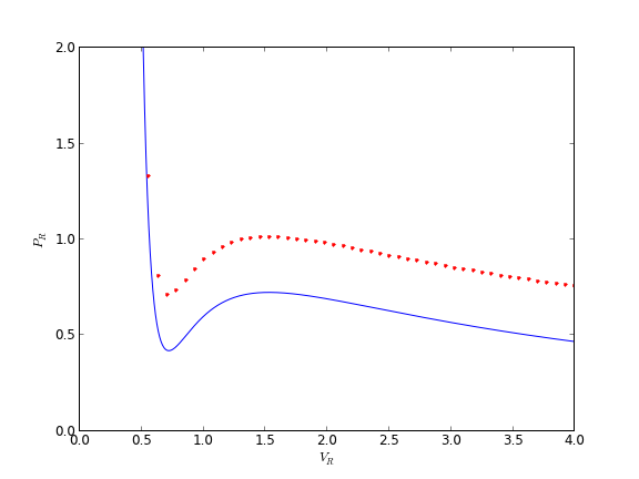
You can see there is disagreement between the analytical solution and numerical solution. The origin of this problem is accuracy at the initial condition, where the derivative is extremely large.

print myode(Po, 0.34)
-53847.3437818

We can increase the tolerance criteria to get a better answer. The defaults in odeint are actually set to 1.49012e-8.

Vspan = np.linspace(0.334, 4)
Po = Prfh(Vspan[0])
P = odeint(myode, Po, Vspan)

# Plot the EOS
plt.plot(Vr,Pr) # analytical solution
plt.plot(Vspan, P[:,0], 'r.')
plt.ylim([0, 2])
plt.xlabel('$V_R$')
plt.ylabel('$P_R$')
plt.savefig('images/ode-vw-3.png')
plt.show()
>>> ... [<matplotlib.lines.Line2D object at 0x1d4dbf10>]
[<matplotlib.lines.Line2D object at 0x1c6e5550>]
(0, 2)
<matplotlib.text.Text object at 0x1d4e31d0>
<matplotlib.text.Text object at 0x1d9d3710>

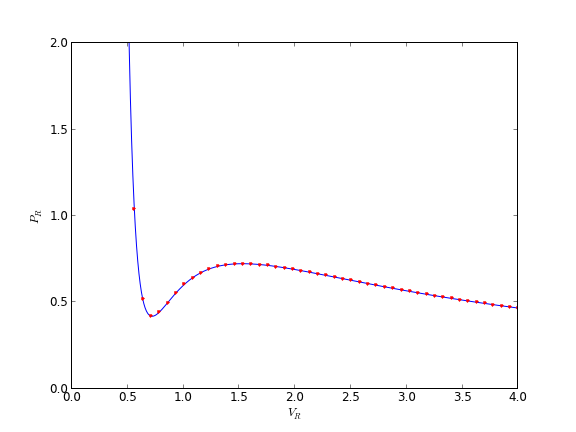
The problem here was the derivative value varied by four orders of magnitude over the integration range, so the default tolerances were insufficient to accurately estimate the numerical derivatives over that range. Tightening the tolerances helped resolve that problem. Another approach might be to split the integration up into different regions. For instance, if instead of starting at Vr = 0.34, which is very close to a sigularity in the van der waal equation at Vr = 1/3, if you start at Vr = 0.5, the solution integrates just fine with the standard tolerances.

Copyright (C) 2013 by John Kitchin. See the License for information about copying.

org-mode source

Discuss on Twitter

Finding minima and maxima in ODE solutions with events

| categories: ode | tags:

Matlab post Today we look at another way to use events in an ode solver. We use an events function to find minima and maxima, by evaluating the ODE in the event function to find conditions where the first derivative is zero, and approached from the right direction. A maximum is when the fisrt derivative is zero and increasing, and a minimum is when the first derivative is zero and decreasing.

We use a simple ODE, \(y' = sin(x)*e^{-0.05x}\), which has minima and maxima.

from pycse import *
import numpy as np

def ode(y, x):
    return np.sin(x) * np.exp(-0.05 * x)

def minima(y, x):
    '''Approaching a minumum, dydx is negatime and going to zero. our event function is increasing'''
    value = ode(y, x)
    direction = 1
    isterminal = False
    return value,  isterminal, direction

def maxima(y, x):
    '''Approaching a maximum, dydx is positive and going to zero. our event function is decreasing'''
    value = ode(y, x)
    direction = -1
    isterminal = False
    return value,  isterminal, direction

xspan = np.linspace(0, 20, 100)

y0 = 0

X, Y, XE, YE, IE = odelay(ode, y0, xspan, events=[minima, maxima])
print IE
import matplotlib.pyplot as plt
plt.plot(X, Y)

# blue is maximum, red is minimum
colors = 'rb'
for xe, ye, ie in zip(XE, YE, IE):
    plt.plot([xe], [ye], 'o', color=colors[ie])

plt.savefig('./images/ode-events-min-max.png')
plt.show()
[1, 0, 1, 0, 1, 0]

Copyright (C) 2013 by John Kitchin. See the License for information about copying.

org-mode source

Discuss on Twitter

Stopping the integration of an ODE at some condition

| categories: ode | tags:

Matlab post In Post 968 we learned how to get the numerical solution to an ODE, and then to use the deval function to solve the solution for a particular value. The deval function uses interpolation to evaluate the solution at other valuse. An alternative approach would be to stop the ODE integration when the solution has the value you want. That can be done in Matlab by using an “event” function. You setup an event function and tell the ode solver to use it by setting an option.

Given that the concentration of a species A in a constant volume, batch reactor obeys this differential equation \(\frac{dC_A}{dt}=- k C_A^2\) with the initial condition \(C_A(t=0) = 2.3\) mol/L and \(k = 0.23\) L/mol/s, compute the time it takes for \(C_A\) to be reduced to 1 mol/L.

from pycse import *
import numpy as np

k = 0.23
Ca0 = 2.3

def dCadt(Ca, t):
    return -k * Ca**2

def stop(Ca, t):
    isterminal = True
    direction = 0
    value = 1.0 - Ca
    return value, isterminal, direction

tspan = np.linspace(0.0, 10.0)

t, CA, TE, YE, IE = odelay(dCadt, Ca0, tspan, events=[stop], full_output=1)

print 'At t = {0:1.2f} seconds the concentration of A is {1:1.2f} mol/L.'.format(t[-1], CA[-1])
At t = 2.46 seconds the concentration of A is 1.00 mol/L.

Copyright (C) 2013 by John Kitchin. See the License for information about copying.

org-mode source

Discuss on Twitter

A simple first order ode evaluated at specific points

| categories: ode | tags:

Matlab post

We have integrated an ODE over a specific time span. Sometimes it is desirable to get the solution at specific points, e.g. at t = [0 0.2 0.4 0.8]; This could be desirable to compare with experimental measurements at those time points. This example demonstrates how to do that.

$$\frac{dy}{dt} = y(t)$$

The initial condition is y(0) = 1.

from scipy.integrate import odeint

y0 = 1
tspan = [0, 0.2, 0.4, 0.8]

def dydt(y, t):
    return y

Y = odeint(dydt, y0, tspan)
print Y[:,0]
[ 1.          1.22140275  1.49182469  2.22554103]

Copyright (C) 2013 by John Kitchin. See the License for information about copying.

org-mode source

Discuss on Twitter
« Previous Page -- Next Page »