The Kitchin Research Group

Matlab post Today we consider how to solve a system of first order, constant coefficient ordinary differential equations using linear algebra. These equations could be solved numerically, but in this case there are analytical solutions that can be derived. The equations we will solve are:

\(y'_1 = -0.02 y_1 + 0.02 y_2\)

\(y'_2 = 0.02 y_1 - 0.02 y_2\)

We can express this set of equations in matrix form as: \(\left[\begin{array}{c}y'_1\\y'_2\end{array}\right] = \left[\begin{array}{cc} -0.02 & 0.02 \\ 0.02 & -0.02\end{array}\right] \left[\begin{array}{c}y_1\\y_2\end{array}\right]\)

The general solution to this set of equations is

\(\left[\begin{array}{c}y_1\\y_2\end{array}\right] = \left[\begin{array}{cc}v_1 & v_2\end{array}\right] \left[\begin{array}{cc} c_1 & 0 \\ 0 & c_2\end{array}\right] \exp\left(\left[\begin{array}{cc} \lambda_1 & 0 \\ 0 & \lambda_2\end{array}\right] \left[\begin{array}{c}t\\t\end{array}\right]\right)\)

where \(\left[\begin{array}{cc} \lambda_1 & 0 \\ 0 & \lambda_2\end{array}\right]\) is a diagonal matrix of the eigenvalues of the constant coefficient matrix, \(\left[\begin{array}{cc}v_1 & v_2\end{array}\right]\) is a matrix of eigenvectors where the \(i^{th}\) column corresponds to the eigenvector of the \(i^{th}\) eigenvalue, and \(\left[\begin{array}{cc} c_1 & 0 \\ 0 & c_2\end{array}\right]\) is a matrix determined by the initial conditions.

In this example, we evaluate the solution using linear algebra. The initial conditions we will consider are \(y_1(0)=0\) and \(y_2(0)=150\).

import numpy as np

A = np.array([[-0.02,  0.02],
              [ 0.02, -0.02]])

# Return the eigenvalues and eigenvectors of a Hermitian or symmetric matrix.
evals, evecs = np.linalg.eigh(A)
print evals
print evecs

>>> ... >>> >>> ... >>> [-0.04  0.  ]
[[ 0.70710678  0.70710678]
 [-0.70710678  0.70710678]]

The eigenvectors are the columns of evecs.

Compute the \(c\) matrix

V*c = Y0

Y0 = [0, 150]

c = np.diag(np.linalg.solve(evecs, Y0))
print c

>>> >>> [[-106.06601718    0.        ]
 [   0.          106.06601718]]

Constructing the solution

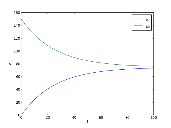
We will create a vector of time values, and stack them for each solution, \(y_1(t)\) and \(Y_2(t)\).

import matplotlib.pyplot as plt

t = np.linspace(0, 100)
T = np.row_stack([t, t])

D = np.diag(evals)

# y = V*c*exp(D*T);
y = np.dot(np.dot(evecs, c), np.exp(np.dot(D, T)))

# y has a shape of (2, 50) so we have to transpose it
plt.plot(t, y.T)
plt.xlabel('t')
plt.ylabel('y')
plt.legend(['$y_1$', '$y_2$'])
plt.savefig('images/ode-la.png')
plt.show()

>>> >>> >>> >>> ... >>> >>> ... [<matplotlib.lines.Line2D object at 0x1d4db950>, <matplotlib.lines.Line2D object at 0x1d4db4d0>]
<matplotlib.text.Text object at 0x1d35fbd0>
<matplotlib.text.Text object at 0x1c222390>
<matplotlib.legend.Legend object at 0x1d34ee90>

Copyright (C) 2013 by John Kitchin. See the License for information about copying.

org-mode source