Finding equilibrium conversion

| categories: nonlinear algebra | tags:

A common problem to solve in reaction engineering is finding the equilibrium conversion.1 A typical problem to solve is the following nonlinear equation:

\(1.44 = \frac{X_e^2}{(1-X_e)^2}\)

To solve this we create a function:

\(f(X_e)=0=1.44 - \frac{X_e^2}{(1-X_e)^2}\)

and use a nonlinear solver to find the value of \(X_e\) that makes this function equal to zero. We have to provide an initial guess. Chemical intuition suggests that the solution must be between 0 and 1, and mathematical intuition suggests the solution might be near 0.5 (which would give a ratio near 1).

Here is our solution.

from scipy.optimize import fsolve

def func(Xe):
    z = 1.44 - (Xe**2)/(1-Xe)**2
    return z

X0 = 0.5
Xe, = fsolve(func, X0)
print('The equilibrium conversion is X = {0:1.2f}'.format(Xe))
The equilibrium conversion is X = 0.55

Copyright (C) 2013 by John Kitchin. See the License for information about copying.

org-mode source

Discuss on Twitter

Counting roots

| categories: nonlinear algebra | tags:

Matlab post The goal here is to determine how many roots there are in a nonlinear function we are interested in solving. For this example, we use a cubic polynomial because we know there are three roots.

$$f(x) = x^3 + 6x^2 - 4x -24$$

1 Use roots for this polynomial

This ony works for a polynomial, it does not work for any other nonlinear function.

import numpy as np
print np.roots([1, 6, -4, -24])
[-6.  2. -2.]

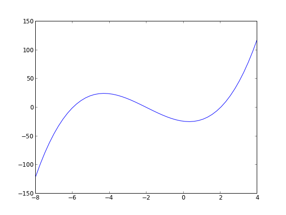
Let us plot the function to see where the roots are.

import numpy as np
import matplotlib.pyplot as plt

x = np.linspace(-8, 4)
y = x**3 + 6 * x**2 - 4*x - 24
plt.plot(x, y)
plt.savefig('images/count-roots-1.png')

Now we consider several approaches to counting the number of roots in this interval. Visually it is pretty easy, you just look for where the function crosses zero. Computationally, it is tricker.

2 method 1

Count the number of times the sign changes in the interval. What we have to do is multiply neighboring elements together, and look for negative values. That indicates a sign change. For example the product of two positive or negative numbers is a positive number. You only get a negative number from the product of a positive and negative number, which means the sign changed.

import numpy as np
import matplotlib.pyplot as plt

x = np.linspace(-8, 4)
y = x**3 + 6 * x**2 - 4*x - 24

print np.sum(y[0:-2] * y[1:-1] < 0)
3

This method gives us the number of roots, but not where the roots are.

3 Method 2

Using events in an ODE solver python can identify events in the solution to an ODE, for example, when a function has a certain value, e.g. f(x) = 0. We can take advantage of this to find the roots and number of roots in this case. We take the derivative of our function, and integrate it from an initial starting point, and define an event function that counts zeros.

$$f'(x) = 3x^2 + 12x - 4$$

with f(-8) = -120

import numpy as np
from pycse import odelay

def fprime(f, x):
    return 3.0 * x**2 + 12.0*x - 4.0

def event(f, x):
    value = f # we want f = 0
    isterminal = False
    direction = 0
    return value, isterminal, direction

xspan = np.linspace(-8, 4)
f0 = -120

X, F, TE, YE, IE = odelay(fprime, f0, xspan, events=[event])
for te, ye in zip(TE, YE):
    print 'root found at x = {0: 1.3f}, f={1: 1.3f}'.format(te, ye)
root found at x = -6.000, f=-0.000
root found at x = -2.000, f=-0.000
root found at x =  2.000, f= 0.000

Copyright (C) 2013 by John Kitchin. See the License for information about copying.

org-mode source

Discuss on Twitter

Method of continuity for nonlinear equation solving

| categories: nonlinear algebra | tags:

Matlab post Adapted from Perry's Chemical Engineers Handbook, 6th edition 2-63.

We seek the solution to the following nonlinear equations:

\(2 + x + y - x^2 + 8 x y + y^3 = 0\)

\(1 + 2x - 3y + x^2 + xy - y e^x = 0\)

In principle this is easy, we simply need some initial guesses and a nonlinear solver. The challenge here is what would you guess? There could be many solutions. The equations are implicit, so it is not easy to graph them, but let us give it a shot, starting on the x range -5 to 5. The idea is set a value for x, and then solve for y in each equation.

import numpy as np
from scipy.optimize import fsolve

import matplotlib.pyplot as plt

def f(x, y):
    return 2 + x + y - x**2 + 8*x*y + y**3;

def g(x, y):
    return 1 + 2*x - 3*y + x**2 + x*y - y*np.exp(x)

x = np.linspace(-5, 5, 500)

@np.vectorize
def fy(x):
    x0 = 0.0
    def tmp(y):
        return f(x, y)
    y1, = fsolve(tmp, x0)
    return y1

@np.vectorize
def gy(x):
    x0 = 0.0
    def tmp(y):
        return g(x, y)
    y1, = fsolve(tmp, x0)
    return y1


plt.plot(x, fy(x), x, gy(x))
plt.xlabel('x')
plt.ylabel('y')
plt.legend(['fy', 'gy'])
plt.savefig('images/continuation-1.png')
>>> >>> >>> >>> ... ... >>> ... ... >>> >>> >>> ... ... ... ... ... ... ... >>> ... ... ... ... ... ... ... >>> >>> /opt/kitchingroup/enthought/epd-7.3-2-rh5-x86_64/lib/python2.7/site-packages/scipy/optimize/minpack.py:152: RuntimeWarning: The iteration is not making good progress, as measured by the 
  improvement from the last ten iterations.
  warnings.warn(msg, RuntimeWarning)
/opt/kitchingroup/enthought/epd-7.3-2-rh5-x86_64/lib/python2.7/site-packages/scipy/optimize/minpack.py:152: RuntimeWarning: The iteration is not making good progress, as measured by the 
  improvement from the last five Jacobian evaluations.
  warnings.warn(msg, RuntimeWarning)
[<matplotlib.lines.Line2D object at 0x1a0c4990>, <matplotlib.lines.Line2D object at 0x1a0c4a90>]
<matplotlib.text.Text object at 0x19d5e390>
<matplotlib.text.Text object at 0x19d61d90>
<matplotlib.legend.Legend object at 0x189df850>
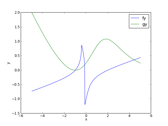
You can see there is a solution near x = -1, y = 0, because both functions equal zero there. We can even use that guess with fsolve. It is disappointly easy! But, keep in mind that in 3 or more dimensions, you cannot perform this visualization, and another method could be required.

def func(X):
    x,y = X
    return [f(x, y), g(x, y)]

print fsolve(func, [-2, -2])
... ... >>> [ -1.00000000e+00   1.28730858e-15]

We explore a method that bypasses this problem today. The principle is to introduce a new variable, \(\lambda\), which will vary from 0 to 1. at \(\lambda=0\) we will have a simpler equation, preferrably a linear one, which can be easily solved, or which can be analytically solved. At \(\lambda=1\), we have the original equations. Then, we create a system of differential equations that start at the easy solution, and integrate from \(\lambda=0\) to \(\lambda=1\), to recover the final solution.

We rewrite the equations as:

\(f(x,y) = (2 + x + y) + \lambda(- x^2 + 8 x y + y^3) = 0\)

\(g(x,y) = (1 + 2x - 3y) + \lambda(x^2 + xy - y e^x) = 0\)

Now, at \(\lambda=0\) we have the simple linear equations:

\(x + y = -2\)

\(2x - 3y = -1\)

These equations are trivial to solve:

x0 = np.linalg.solve([[1., 1.], [2., -3.]],[ -2, -1])
print x0
[-1.4 -0.6]

We form the system of ODEs by differentiating the new equations with respect to \(\lambda\). Why do we do that? The solution, (x,y) will be a function of \(\lambda\). From calculus, you can show that:

\(\frac{\partial f}{\partial x}\frac{\partial x}{\partial \lambda}+\frac{\partial f}{\partial y}\frac{\partial y}{\partial \lambda}=-\frac{\partial f}{\partial \lambda}\)

\(\frac{\partial g}{\partial x}\frac{\partial x}{\partial \lambda}+\frac{\partial g}{\partial y}\frac{\partial y}{\partial \lambda}=-\frac{\partial g}{\partial \lambda}\)

Now, solve this for \(\frac{\partial x}{\partial \lambda}\) and \(\frac{\partial y}{\partial \lambda}\). You can use Cramer's rule to solve for these to yield:

\begin{eqnarray} \ \frac{\partial x}{\partial \lambda} &=& \frac{\partial f/\partial y \partial g/\partial \lambda - \partial f/\partial \lambda \partial g/\partial y}{\partial f/\partial x \partial g/\partial y - \partial f/\partial y \partial g/\partial x } \\\\ \frac{\partial y}{\partial \lambda} &=& \frac{\partial f/\partial \lambda \partial g/\partial x - \partial f/\partial x \partial g/\partial \lambda}{\partial f/\partial x \partial g/\partial y - \partial f/\partial y \partial g/\partial x } \end{eqnarray} For this set of equations: \begin{eqnarray} \ \partial f/\partial x &=& 1 - 2\lambda x + 8\lambda y \\\\ \partial f/\partial y &=& 1 + 8 \lambda x + 3 \lambda y^2 \\\\ \partial g/\partial x &=& 2 + 2 \lambda x + \lambda y - \lambda y e^x\\\\ \partial g/\partial y &=& -3 + \lambda x - \lambda e^x \end{eqnarray}

Now, we simply set up those two differential equations on \(\frac{\partial x}{\partial \lambda}\) and \(\frac{\partial y}{\partial \lambda}\), with the initial conditions at \(\lambda = 0\) which is the solution of the simpler linear equations, and integrate to \(\lambda = 1\), which is the final solution of the original equations!

def ode(X, LAMBDA):
    x,y = X
    pfpx = 1.0 - 2.0 * LAMBDA * x + 8 * LAMBDA * y
    pfpy = 1.0 + 8.0 * LAMBDA * x + 3.0 * LAMBDA * y**2
    pfpLAMBDA = -x**2 + 8.0 * x * y + y**3;
    pgpx = 2. + 2. * LAMBDA * x + LAMBDA * y - LAMBDA * y * np.exp(x)
    pgpy = -3. + LAMBDA * x - LAMBDA * np.exp(x)
    pgpLAMBDA = x**2 + x * y - y * np.exp(x);
    dxdLAMBDA = (pfpy * pgpLAMBDA - pfpLAMBDA * pgpy) / (pfpx * pgpy - pfpy * pgpx)
    dydLAMBDA = (pfpLAMBDA * pgpx - pfpx * pgpLAMBDA) / (pfpx * pgpy - pfpy * pgpx) 
    dXdLAMBDA = [dxdLAMBDA, dydLAMBDA]
    return dXdLAMBDA


from scipy.integrate import odeint

lambda_span = np.linspace(0, 1, 100)

X = odeint(ode, x0, lambda_span)

xsol, ysol = X[-1]
print 'The solution is at x={0:1.3f}, y={1:1.3f}'.format(xsol, ysol)
print f(xsol, ysol), g(xsol, ysol)
... ... ... ... ... ... ... ... ... >>> >>> >>> >>> >>> >>> >>> The solution is at x=-1.000, y=0.000
-1.27746598808e-06 -1.15873819107e-06

You can see the solution is somewhat approximate; the true solution is x = -1, y = 0. The approximation could be improved by lowering the tolerance on the ODE solver. The functions evaluate to a small number, close to zero. You have to apply some judgment to determine if that is sufficiently accurate. For instance if the units on that answer are kilometers, but you need an answer accurate to a millimeter, this may not be accurate enough.

This is a fair amount of work to get a solution! The idea is to solve a simple problem, and then gradually turn on the hard part by the lambda parameter. What happens if there are multiple solutions? The answer you finally get will depend on your \(\lambda=0\) starting point, so it is possible to miss solutions this way. For problems with lots of variables, this would be a good approach if you can identify the easy problem.

Copyright (C) 2013 by John Kitchin. See the License for information about copying.

org-mode source
Discuss on Twitter

Calculating a bubble point pressure of a mixture

| categories: nonlinear algebra | tags: thermodynamics

Matlab post

Adapted from http://terpconnect.umd.edu/~nsw/ench250/bubpnt.htm (dead link)

We previously learned to read a datafile containing lots of Antoine coefficients into a database, and use the coefficients to estimate vapor pressure of a single compound. Here we use those coefficents to compute a bubble point pressure of a mixture.

The bubble point is the temperature at which the sum of the component vapor pressures is equal to the the total pressure. This is where a bubble of vapor will first start forming, and the mixture starts to boil.

Consider an equimolar mixture of benzene, toluene, chloroform, acetone and methanol. Compute the bubble point at 760 mmHg, and the gas phase composition. The gas phase composition is given by: \(y_i = x_i*P_i/P_T\).

import numpy as np
from scipy.optimize import fsolve

# load our thermodynamic data
data = np.loadtxt('data/antoine_data.dat',
                  dtype=[('id', np.int),
                         ('formula', 'S8'),
                         ('name', 'S28'),
                         ('A', np.float),
                         ('B', np.float),
                         ('C', np.float),
                         ('Tmin', np.float),
                         ('Tmax', np.float),
                         ('??', 'S4'),
                         ('?', 'S4')],
                  skiprows=7)

compounds = ['benzene', 'toluene', 'chloroform', 'acetone', 'methanol']

# extract the data we want
A = np.array([data[data['name'] == x]['A'][0] for x in compounds])
B = np.array([data[data['name'] == x]['B'][0] for x in compounds])
C = np.array([data[data['name'] == x]['C'][0] for x in compounds])
Tmin = np.array([data[data['name'] == x]['Tmin'][0] for x in compounds])
Tmax = np.array([data[data['name'] == x]['Tmax'][0] for x in compounds])


# we have an equimolar mixture
x = np.array([0.2, 0.2, 0.2, 0.2, 0.2])

# Given a T, we can compute the pressure of each species like this:

T = 67 # degC
P = 10**(A - B / (T + C))
print P
print np.dot(x, P)  # total mole-fraction weighted pressure

Tguess = 67
Ptotal = 760

def func(T):
    P = 10**(A - B / (T + C))
    return Ptotal - np.dot(x, P)
    
Tbubble, = fsolve(func, Tguess)

print 'The bubble point is {0:1.2f} degC'.format(Tbubble)

# double check answer is in a valid T range
if np.any(Tbubble < Tmin) or np.any(Tbubble > Tmax):
    print 'T_bubble is out of range!'

# print gas phase composition
y = x * 10**(A - B / (Tbubble + C))/Ptotal

for cmpd, yi in zip(compounds, y):
    print 'y_{0:<10s} = {1:1.3f}'.format(cmpd, yi)
[  498.4320267    182.16010994   898.31061294  1081.48181768   837.88860027]
699.654633507
The bubble point is 69.46 degC
y_benzene    = 0.142
y_toluene    = 0.053
y_chloroform = 0.255
y_acetone    = 0.308
y_methanol   = 0.242

Copyright (C) 2013 by John Kitchin. See the License for information about copying.

org-mode source

Discuss on Twitter

Solving CSTR design equations

| categories: nonlinear algebra | tags: reaction engineering

Given a continuously stirred tank reactor with a volume of 66,000 dm^3 where the reaction \(A \rightarrow B\) occurs, at a rate of \(-r_A = k C_A^2\) (\(k=3\) L/mol/h), with an entering molar flow of F_{A0} = 5 mol/h and a volumetric flowrate of 10 L/h, what is the exit concentration of A?

From a mole balance we know that at steady state \(0 = F_{A0} - F_A + V r_A\). That equation simply states the sum of the molar flow of A in in minus the molar flow of A out plus the molar rate A is generated is equal to zero at steady state. This is directly the equation we need to solve. We need the following relationship:

  1. \(F_A = v0 C_A\)
from scipy.optimize import fsolve

Fa0 = 5.0
v0 = 10.

V = 66000.0  # reactor volume L^3
k = 3.0      # rate constant L/mol/h

def func(Ca):
    "Mole balance for a CSTR. Solve this equation for func(Ca)=0"
    Fa = v0 * Ca     # exit molar flow of A
    ra = -k * Ca**2  # rate of reaction of A L/mol/h
    return Fa0 - Fa + V * ra

# CA guess that that 90 % is reacted away
CA_guess = 0.1 * Fa0 / v0
CA_sol, = fsolve(func, CA_guess)

print 'The exit concentration is {0} mol/L'.format(CA_sol)
The exit concentration is 0.005 mol/L

It is a little confusing why it is necessary to put a comma after the CA_sol in the fsolve command. If you do not put it there, you get brackets around the answer.

Copyright (C) 2013 by John Kitchin. See the License for information about copying.

org-mode source

Discuss on Twitter
« Previous Page -- Next Page »