Using autograd to plot implicit functions
Posted October 02, 2019 at 09:30 PM | categories: autograd, implicit-function, nonlinear-algebra | tags:
Consider the solution to these equations (adapted from https://www.mathworks.com/help/optim/ug/fsolve.html):
\(e^{-e^{-(x_1 + x_2)}} = x_2 (1 + x_1^2)\)
and
\(x_1 \cos(x_2) + x_2 \sin(x_1) = 1/2\)
It is not clear how many solutions there are to this set of equations, or what you should guess for the initial guess. Usually, the best way to see where a solution might be is to plot the equations and see where they intersect. These equations are implicit though, and it is not easy to plot them because we cannot solve for \(x_2\) in terms of \(x_1\) in either case. Here we explore a strategy to get plots so we can see where solutions could be.
The idea is that we find one solution to each equation independently. Then, we derive a differential equation for each equation so we can integrate it to find the curve that is defined by the implicit function. First, we find a solution for each equation. We guess a value for \(x_2\) and then find the value of \(x_1\) that solves each equation independently.
import autograd.numpy as np
from scipy.optimize import fsolve

def f1(x1, x2):
    return np.exp(-np.exp(-(x1 + x2))) - x2 * (1 + x1**2)

def f2(x1, x2):
    return x1 * np.cos(x2) + x2 * np.sin(x1) - 0.5

x2_1 = 0.6
x1_1, = fsolve(f1, 0, args=(x2_1,))
print('f1: ', x1_1, x2_1)

x2_2 = 1.0
x1_2, = fsolve(f2, 0 ,args=(x2_2,))
print('f2: ', x1_2, x2_2)
f1: 0.08638978040861575 0.6 f2: 0.32842406163614396 1.0
Next, we need a differential equation that is \(dx_2/dx_1\). If we had that, we could just integrate it from one of the starting points above, and get the curve we want. The functions are implicit, so we have to use the implicit derivative, which for the first equation is \(dx_2/dx_1 = -df1/dx_1 / df1/dx_2\). We will get these gradients from autograd. Then, we just integrate the solution. Here we do this for the first equation.
from scipy.integrate import solve_ivp
from autograd import grad

df1dx1 = grad(f1, 0)
df1dx2 = grad(f1, 1)

def dx2dx1_1(x1, x2):
    return -df1dx1(x1, x2) / df1dx2(x1, x2)

x1_span = (x1_1, 1)
x2_0 = (x2_1, )
sol1 = solve_ivp(dx2dx1_1, x1_span, x2_0, max_step=0.1)
And then, we do it for the second equation.
df2dx1 = grad(f2, 0)
df2dx2 = grad(f2, 1)

def dx2dx1_2(x1, x2):
    return -df2dx1(x1, x2) / df2dx2(x1, x2)

x1_span = (x1_2, 1)
x2_0 = (x2_2, )
sol2 = solve_ivp(dx2dx1_2, x1_span, x2_0, max_step=0.1)
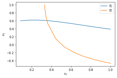
Finally, we plot the two solutions.
%matplotlib inline
import matplotlib.pyplot as plt
plt.plot(sol1.t, sol1.y.T)
plt.plot(sol2.t, sol2.y.T)
plt.xlabel('$x_1$')
plt.ylabel('$x_2$')
plt.legend(['f1', 'f2'])
<Figure size 432x288 with 1 Axes>

You can see now that in this range, there is only one intersection, i.e. one solution, and it is near \(x_1=0.4, x_2=0.6\). We can finally use that as an initial guess to find the only solution in this region, with confidence we are not missing any solutions.
def objective(X):
    x1, x2 = X
    return [f1(x1, x2), f2(x1, x2)]

fsolve(objective, [0.4, 0.6])
array([0.35324662, 0.60608174])
That is the same solution as reported at the Matlab site. Another use of autograd for the win here.
Copyright (C) 2019 by John Kitchin. See the License for information about copying.
Org-mode version = 9.2.3