The Kitchin Research Group

This paper describes how sensitivity analysis requires access to the derivatives of a function. Say, for example we have a function describing the time evolution of the concentration of species A:

\([A] = \frac{[A]_0}{k_1 + k_{-1}} (k_1 e^{(-(k_1 _ k_{-1})t)} + k_{-1})\)

The local sensitivity of the concentration of A to the parameters \(k1\) and \(k_1\) are defined as \(\frac{\partial A}{\partial k1}\) and \(\frac{\partial A}{\partial k_1}\). Our goal is to plot the sensitivity as a function of time. We could derive those derivatives, but we will use auto-differentiation instead through the autograd package. Here we import numpy from the autograd package and plot the function above.

import autograd.numpy as np

A0 = 1.0

def A(t, k1, k_1):
    return A0 / (k1 + k_1) * (k1 * np.exp(-(k1 + k_1) * t) + k_1)

%matplotlib inline
import matplotlib.pyplot as plt

t = np.linspace(0, 0.5)

k1 = 3.0
k_1 = 3.0
plt.plot(t, A(t, k1, k_1))
plt.xlim([0, 0.5])
plt.ylim([0, 1])
plt.xlabel('t')
plt.ylabel('A')

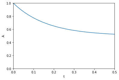
The figure above reproduces Fig. 1 from the paper referenced above. Next, we use autograd to get the derivatives. This is subtly different than our previous post. First, we need the derivative of the function with respect to the second and third arguments; the default is the first argument. Second, we want to evaluate this derivative at each time value. We use the jacobian function in autograd to get these. This is different than grad, which will sum up the derivatives at each time. That might be useful for regression, but not for sensitivity analysis. Finally, to reproduce Figure 2a, we plot the absolute value of the sensitivities.

from autograd import jacobian

dAdk1 = jacobian(A, 1)
dAdk_1 = jacobian(A, 2)

plt.plot(t, np.abs(dAdk1(t, k1, k_1)))
plt.plot(t, np.abs(dAdk_1(t, k1, k_1)))
plt.xlim([0, 0.5])
plt.ylim([0, 0.1])
plt.xlabel('t')
plt.legend(['$S_{k1}$', '$S_{k\_1}$'])

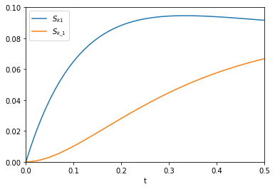
That looks like the figure in the paper. To summarize the main takeaway, autograd enabled us to readily compute derivatives without having to derive them manually. There was a little subtlety in choosing jacobian over grad or elementwise_grad but once you know what these do, it seems reasonable. It is important to import the wrapped numpy first, to enable autograd to do its work. All the functions here are pretty standard, so everything worked out of the box. We should probably be using autograd, or something like it for more things in science!

Copyright (C) 2017 by John Kitchin. See the License for information about copying.

org-mode source

Org-mode version = 9.1.2

In molecular simulation we often use a potential to compute the total energy of a system. For example, we might use something simple like a Lennard-Jones potential. If we have a potential function, e.g. \(E = V(R)\) where \(R\) are the positions of the atoms, then we know the forces on the atoms are defined by \(f = -\frac{dV}{dR}\). For simple functions, you can derive the derivative pretty easily, but these functions quickly get complicated. In this post, we consider automatic differentiation as implemented by autograd. This is neither symbolic nor numerical differentiation. The gist is that the program uses the chain rule to evaluate derivatives. Here we do not delve into how it is done, we just see how it might help us in molecular simulation.

For reference, here is a result from the LennardJones calculator in ASE.

from ase.calculators.lj import LennardJones
from ase.cluster.icosahedron import Icosahedron

atoms = Icosahedron('Ar', noshells=2, latticeconstant=3)
atoms.set_calculator(LennardJones())

atoms.rattle(0.5)
print('LJ: ', atoms.get_potential_energy())

('LJ: ', -3.3553466825679812)

First, we define a function for the Lennard-Jones potential. I adapted the code here to implement a function that calculates the Lennard-Jones energy for a cluster of atoms with no periodic boundary conditions. Instead of using numpy directly, we import it from the autograd package which puts thin wrappers around the functions to enable the derivative calculations.

import autograd.numpy as np

def energy(positions):
    "Compute the energy of a Lennard-Jones system."
    natoms = len(positions)

    sigma = 1.0
    epsilon = 1.0
    rc = 3 * sigma

    e0 = 4 * epsilon * ((sigma / rc)**12 - (sigma / rc)**6)
    energy = 0.0
    for a1 in range(natoms):
        for j in range(a1 + 1, natoms):
            r2 = np.sum((positions[a1] - positions[j])**2)
            if r2 <= rc**2:
                c6 = (sigma**2 / r2)**3
                energy -= e0 
                c12 = c6**2
                energy += 4 * epsilon * (c12 - c6)

    return energy

Here is our function in action, and it produces the same result as the ASE calculator. So far there is nothing new.

print('our func: ', energy(atoms.positions))

('our func: ', -3.3553466825679803)

Now, we look at the forces from the ASE calculator. If you look at the ASE code you will see that the formula for forces was analytically derived and accumulated in the loop.

np.set_printoptions(precision=3, suppress=True)
print(atoms.get_forces())

[[ 0.545  1.667  0.721]
 [-0.068  0.002  0.121]
 [-0.18   0.018 -0.121]
 [ 0.902 -0.874 -0.083]
 [ 0.901 -0.937 -1.815]
 [ 0.243 -0.19   0.063]
 [-0.952 -1.776 -0.404]
 [-0.562  1.822  1.178]
 [-0.235  0.231  0.081]
 [-0.023  0.204 -0.294]
 [ 0.221 -0.342 -0.425]
 [-5.385 -6.017  1.236]
 [ 4.593  6.193 -0.258]]

Now we look at how to use autograd for this purpose. We want an element-wise gradient of the total energy with respect to the positions. autograd returns functions, so we wrap it in another function so we can take the negative of that function.

from autograd import elementwise_grad

def forces(pos):
    dEdR = elementwise_grad(energy)
    return -dEdR(pos)

print(forces(atoms.positions))

[[ 0.545  1.667  0.721]
 [-0.068  0.002  0.121]
 [-0.18   0.018 -0.121]
 [ 0.902 -0.874 -0.083]
 [ 0.901 -0.937 -1.815]
 [ 0.243 -0.19   0.063]
 [-0.952 -1.776 -0.404]
 [-0.562  1.822  1.178]
 [-0.235  0.231  0.081]
 [-0.023  0.204 -0.294]
 [ 0.221 -0.342 -0.425]
 [-5.385 -6.017  1.236]
 [ 4.593  6.193 -0.258]]

Here we show the results are the same from both approaches.

print(np.allclose(atoms.get_forces(), forces(atoms.positions)))

True

Wow. We got forces without deriving a derivative, or using numerical finite differences, across loops, and conditionals. That is pretty awesome. You can easily modify the potential function now, without the need to rederive the force derivatives! This is an idea worth exploring further. In principle, it should be possible to include periodic boundary conditions and use autograd to compute stresses too. Maybe that will be a future post.

Copyright (C) 2017 by John Kitchin. See the License for information about copying.

org-mode source

Org-mode version = 9.1.2