More auto-differentiation goodness for science and engineering

| categories: autograd, python | tags:

In this post I continue my investigations in the use of auto-differentiation via autograd in scientific and mathematical programming. The main focus of today is using autograd to get derivatives that either have mathematical value, eg. accelerating root finding, or demonstrating mathematical rules, or scientific value, e.g. the derivative is related to a property, or illustrates some constraint.

All the code in this post relies on these imports:

import autograd.numpy as np
from autograd import grad, jacobian

In the following sections I explore some applications in calculus, root-finding, materials and thermodynamics.

1 Showing mixed partial derivatives are equal

In calculus, we know that if we have a well-behaved function \(f(x, y)\), then it should be true that \(\frac{\partial^2f}{\partial x \partial y} = \frac{\partial^2f}{\partial y \partial y}\).

Here we use autograd to compute the mixed partial derivatives and show for 10 random points that this statement is true. This doesnt' prove it for all points, of course, but it is easy to prove for any point of interest.

def f(x, y):
    return x * y**2

dfdx = grad(f)
d2fdxdy = grad(dfdx, 1)

dfdy = grad(f, 1)
d2fdydx = grad(dfdy)

x = np.random.rand(10)
y = np.random.rand(10)

T = [d2fdxdy(x1, y1) == d2fdydx(x1, y1) for x1, y1 in zip(x, y)]

print(np.all(T))

True

2 Root finding with jacobians

fsolve often works fine without access to derivatives. In this example from here, we solve a set of equations with two variables, and it takes 21 iterations to reach the solution.

from scipy.optimize import fsolve

def f(x):
    return np.array([x[1] - 3*x[0]*(x[0]+1)*(x[0]-1),
                     .25*x[0]**2 + x[1]**2 - 1])


ans, info, flag, msg = fsolve(f, (0.5, 0.5), full_output=1)
print(ans)
print(info['nfev'])

[ 1.117 0.83 ] 21

If we add the jacobian, we get the same result with only 15 iterations, about 1/3 fewer iterations. If the iterations are expensive, this might save a lot of time.

df = jacobian(f)
x0 = np.array([0.5, 0.5])

ans, info, flag, msg  = fsolve(f, x0, fprime=df, full_output=1)
print(ans)
print(info['nfev'])

[ 1.117 0.83 ] 15

There is a similar example provided by autograd.

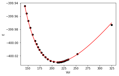
3 Getting the pressure from a solid equation of state

In this post we described how to fit a solid equation of state to describe the energy of a solid under isotropic strain. Now, we can readily compute the pressure at a particular volume from the equation:

\(P = -\frac{dE}{dV}\)

We just need the derivative of this equation:

\(E = E_0+\frac{B_0 V}{B'_0}\left[\frac{(V_0/V)^{B'_0}}{B'_0-1}+1\right]-\frac{V_0 B_0}{B'_0-1}\)

or we use autograd to get it for us.

E0, B0, BP, V0 = -56.466,   0.49,    4.753,  16.573

def Murnaghan(vol):
    E = E0 + B0 * vol / BP * (((V0 / vol)**BP) / (BP - 1.0) + 1.0) - V0 * B0 / (BP - 1.)
    return E

def P(vol):
    dEdV = grad(Murnaghan)
    return -dEdV(vol) * 160.21773  # in Gpa

print(P(V0)) # Pressure at the minimum
print(P(0.99 * V0))  # Compressed
4.44693531998e-15
0.808167684691

So it takes positive pressure to compress the system, as expected, and at the minimum the pressure is equal to zero. Seems pretty clear autograd is better than deriving the required pressure derivative.

4 Deriving activity coefficients and demonstration of the Gibbs-Duhem relation

Thermodynamics tells us that in a binary mixture the following is true:

\(0 = x_1 \frac{d \ln \gamma_1}{dx_1} + (1 - x_1) \frac{d \ln \gamma_2}{dx_1}\)

In other words, the activity coefficients of the two species can't be independent.

Suppose we have the Margules model for the excess free energy:

\(G^{ex}/RT = n x_1 (1 - x_1) (A_{21} x_1 + A_{12} (1 - x_1))\)

where \(n = n_1 + n_2\), and \(x_1 = n1 / n\), and \(x_2 = n_2 / n\).

From this expression, we know:

\(\ln \gamma_1 = \frac{\partial G_{ex}/RT}{\partial n_1}\)

and

\(\ln \gamma_2 = \frac{\partial G_{ex}/RT}{\partial n_2}\)

It is also true that (the Gibbs-Duhem equation):

\(0 = x_1 \frac{d \ln \gamma_1}{d n_1} + x_2 \frac{d \ln \gamma_2}{d n_1}\)

Here we will use autograd to get these derivatives, and demonstrate the Gibbs-Duhem eqn holds for this excess Gibbs energy model.

A12, A21 = 2.04, 1.5461  # Acetone/water https://en.wikipedia.org/wiki/Margules_activity_model

def GexRT(n1, n2):
    n = n1 + n2
    x1 = n1 / n
    x2 = n2 / n
    return n * x1 * x2 * (A21 * x1 + A12 * x2)

lngamma1 = grad(GexRT)     # dGex/dn1
lngamma2 = grad(GexRT, 1)  # dGex/dn2

n1, n2 = 1.0, 2.0
n = n1 + n2
x1 = n1 / n
x2 = n2 / n

# Evaluate the activity coefficients
print('AD:         ',lngamma1(n1, n2), lngamma2(n1, n2))

# Compare that to these analytically derived activity coefficients
print('Analytical: ', (A12 + 2 * (A21 - A12) * x1) * x2**2, (A21 + 2 * (A12 - A21) * x2) * x1**2)

# Demonstration of the Gibbs-Duhem rule
dg1 = grad(lngamma1)
dg2 = grad(lngamma2)

n = 1.0 # Choose a basis number of moles
x1 = np.linspace(0, 1)
x2 = 1 - x1
n1 = n * x1
n2 = n - n1

GD = [_x1 * dg1(_n1, _n2) + _x2 * dg2(_n1, _n2)
      for _x1, _x2, _n1, _n2 in zip(x1, x2, n1, n2)]

print(np.allclose(GD, np.zeros(len(GD))))
('AD:         ', 0.76032592592592585, 0.24495925925925932)
('Analytical: ', 0.760325925925926, 0.24495925925925924)
True

That is pretty compelling. The autograd derivatives are much easier to code than the analytical solutions (which also had to be derived). You can also see that the Gibbs-Duhem equation is satisfied for this model, at least with a reasonable tolerance for the points we evaluated it at.

5 Summary

Today we examined four ways to use autograd in scientific or mathematical programs to replace the need to derive derivatives by hand. The main requirements for this to work are that you use the autograd.numpy module, and only the functions in it that are supported. It is possible to add your own functions (described in the tutorial) if needed. It seems like there are a lot of opportunities for scientific programming for autograd.

Copyright (C) 2017 by John Kitchin. See the License for information about copying.

org-mode source

Org-mode version = 9.1.2

Discuss on Twitter

Timing Lennard-Jones implementations - ASE vs autograd

| categories: lennardjones, autograd, python | tags:

Table of Contents

In a comment on this post Konrad Hinsen asked if the autograd forces on a Lennard-Jones potential would be useable in production. I wasn't sure, and was suspicious that analytical force functions would be faster. It turns out to not be so simple. In this post, I attempt to do some timing experiments for comparison. These are tricky to do right, and in a meaningful way, so I will start by explaining what is tricky and why I think the results are meaningful.

The ASE calculators cache their results, and return the cached results after the first run. We will do these on a 13-atom icosahedron cluster.

from ase.calculators.lj import LennardJones
from ase.cluster.icosahedron import Icosahedron

atoms = Icosahedron('Ar', noshells=2, latticeconstant=3)
atoms.set_calculator(LennardJones())

import time
t0 = time.time()
print('energy: ', atoms.get_potential_energy())
print(' time: ', time.time() - t0)
print()

t0 = time.time()
print('energy: ', atoms.get_potential_energy())
print(' time: ', time.time() - t0)
print()

atoms.calc.results = {}
t0 = time.time()
print('energy: ', atoms.get_potential_energy())
print('time: ', time.time() - t0)
energy:  -1.25741774649
 time:  0.0028629302978515625

energy:  -1.25741774649
 time:  0.00078582763671875

energy:  -1.25741774649
time:  0.0031850337982177734

Note the approximate order of magnitude reduction in elapsed time for the second call. After that, we reset the calculator results, and the time goes back up. So, we have to incorporate that into our timing. Also, in the ASE calculator, the forces are simultaneously calculated. There isn't a way to separate the calls. I am going to use the timeit feature in Ipython for the timing. I don't have a lot of control over what else is running on my machine, so I have observed some variability in the timing results. Finally, I am running these on a MacBook Air.

%%timeit
atoms.get_potential_energy()
atoms.calc.results = {} # this resets it so it runs each time. Otherwise, we get cached results

1.46 ms ± 107 µs per loop (mean ± std. dev. of 7 runs, 1000 loops each)

That seems like a surprisingly long time. If you neglect the calculator reset, it looks about 10 times faster because the cache lookup is fast!

Let's compare that to an implementation of the Lennard-Jones potential similar to the last time. This implementation differs from the first one I blogged about. This one is fully vectorized. It still does not support periodic boundary conditions though. This version may be up to 10 times faster than the previous version. I haven't tested this very well, I only assured it gives the same energy as ASE for the example in this post.

import autograd.numpy as np

def energy(positions):
    "Compute the energy of a Lennard-Jones system."
    
    sigma = 1.0
    epsilon = 1.0
    rc = 3 * sigma

    e0 = 4 * epsilon * ((sigma / rc)**12 - (sigma / rc)**6)
    
    natoms = len(positions)
    # These are the pairs of indices we need to compute distances for.
    a, b = np.triu_indices(natoms, 1)

    d = positions[a] - positions[b]
    r2 = np.sum(d**2, axis=1)
    c6 = np.where(r2 <= rc**2, (sigma**2 / r2)**3, np.zeros_like(r2))
    
    energy = -e0 * (c6 != 0.0).sum()
    c12 = c6**2
    energy += np.sum(4 * epsilon * (c12 - c6))
    
    return energy

# Just to check we get the same answer
print(energy(atoms.positions))

-1.25741774649

The energy looks good. For timing, we store the positions in a variable, in case there is any lookup time, since this function only needs an array.

pos = atoms.positions

There is no caching to worry about here, we can just get the timing.

%%timeit
energy(pos)

82.2 µs ± 2.85 µs per loop (mean ± std. dev. of 7 runs, 10000 loops each)

Wow, that is a lot faster than the ASE implementation. Score one for vectorization.

print('Vectorized is {0:1.1f} times faster than ASE at energy.'.format(1.46e-3 / 82.5e-6))
Vectorized is 17.7 times faster than ASE at energy.

Yep, a fully vectorized implementation is a lot faster than the ASE version which uses loops. So far the difference has nothing to do with autograd.

1 Timing on the forces

The forces are where derivatives are important, and it is a reasonable question of whether hand-coded derivatives are faster or slower than autograd derivatives. We first look at the forces from ASE. The analytical forces take about the same time as the energy, which is not surprising. The same work is done for both of them.

np.set_printoptions(precision=3, suppress=True)
print(atoms.get_forces())
[[-0.    -0.    -0.   ]
 [-0.296 -0.     0.183]
 [-0.296 -0.    -0.183]
 [ 0.296 -0.     0.183]
 [ 0.296 -0.    -0.183]
 [ 0.183 -0.296 -0.   ]
 [-0.183 -0.296  0.   ]
 [ 0.183  0.296 -0.   ]
 [-0.183  0.296  0.   ]
 [-0.     0.183 -0.296]
 [ 0.    -0.183 -0.296]
 [-0.     0.183  0.296]
 [ 0.    -0.183  0.296]]

%%timeit
atoms.get_forces()
atoms.calc.results = {}
1.22 ms ± 38.7 µs per loop (mean ± std. dev. of 7 runs, 1000 loops each)

Here is our auto-differentiated force function.

from autograd import elementwise_grad

def forces(pos):
    dEdR = elementwise_grad(energy)
    return -dEdR(pos)

Let's just check the forces for consistency.

print(forces(atoms.positions))

print(np.allclose(forces(atoms.positions), atoms.get_forces()))
[[-0.    -0.    -0.   ]
 [-0.296 -0.     0.183]
 [-0.296 -0.    -0.183]
 [ 0.296 -0.     0.183]
 [ 0.296 -0.    -0.183]
 [ 0.183 -0.296 -0.   ]
 [-0.183 -0.296  0.   ]
 [ 0.183  0.296 -0.   ]
 [-0.183  0.296  0.   ]
 [-0.     0.183 -0.296]
 [ 0.    -0.183 -0.296]
 [-0.     0.183  0.296]
 [ 0.    -0.183  0.296]]
True

Those all look the same, so now performance for that:

%%timeit 

forces(pos)
727 µs ± 47.1 µs per loop (mean ± std. dev. of 7 runs, 1000 loops each)

This is faster than the ASE version. I suspect that it is largely because of the faster, vectorized algorithm overall.

print('autograd is {0:1.1f} times faster than ASE on forces.'.format(1.22e-3 / 727e-6))
autograd is 1.7 times faster than ASE on forces.

autograd forces are consistently 2-6 times faster than the ASE implementation. It could be possible to hand-code a faster function for the forces, if it was fully vectorized. I spent a while seeing what would be required for that, and it is not obvious how to do that. Any solution that uses loops will be slower I think.

This doesn't directly answer the question of whether this can work in production. Everything is still written in Python here, which might limit the size and length of calculations you can practically do. With the right implementation though, it looks promising.

Copyright (C) 2017 by John Kitchin. See the License for information about copying.

org-mode source

Org-mode version = 9.1.2

Discuss on Twitter

Training the ASE Lennard-Jones potential to DFT calculations

| categories: autograd, python | tags:

The Atomic Simulation Environment provides several useful calculators with configurable parameters. For example, the Lennard-Jones potential has two adjustable parameters, σ and ε. I have always thought it would be useful to be able to fit one of these potentials to a reference database, e.g. a DFT database.

I ran a series of DFT calculations of bulk Ar in different crystal structures, at different volumes and saved them in an ase database (argon.db ). We have five crystal structures at three different volumes. Within each of those sets, I rattled the atoms a bunch of times and calculated the energies. Here is the histogram of energies we have to work with:

%matplotlib inline
import matplotlib.pyplot as plt

import ase.db
db = ase.db.connect('argon.db')

known_energies = [row.energy for row in db.select()]
plt.hist(known_energies, 20)
plt.xlabel('Energy')

What I would really like is a set of Lennard-Jones parameters that describe this data. It only recently occurred to me that we just need to define a function that takes the LJ parameters and computes energies for a set of configurations. Then we create a second objective function we can use in a minimization. Here is how we can implement that idea:

import numpy as np
from scipy.optimize import fmin
from ase.calculators.lj import LennardJones

def my_lj(pars):
    epsilon, sigma = pars
    calc = LennardJones(sigma=sigma, epsilon=epsilon)
    all_atoms = [row.toatoms() for row in db.select()]
    [atoms.set_calculator(calc) for atoms in all_atoms]
    predicted_energies = np.array([atoms.get_potential_energy() for atoms in all_atoms])
    return predicted_energies

def objective(pars):
    known_energies = np.array([row.energy for row in db.select()])
    err = known_energies - my_lj(pars)
    return np.mean(err**2)

LJ_pars = fmin(objective, [0.005, 3.5])        
print(LJ_pars)
Optimization terminated successfully.
         Current function value: 0.000141
         Iterations: 28
         Function evaluations: 53
[ 0.00593014  3.73314611]

Now, let's see how well we do with that fit.

plt.subplot(121)

calc = LennardJones(epsilon=LJ_pars[0], sigma=LJ_pars[1])

for structure, spec in [('fcc', 'b.'),
                        ('hcp', 'r.'),
                        ('bcc', 'g.'),
                        ('diamond', 'gd'),
                        ('sc', 'bs')]:

    ke, pe = [], []
    for row in db.select(structure=structure):
        ke += [row.energy]
        atoms = row.toatoms()
        atoms.set_calculator(calc)
        pe += [atoms.get_potential_energy()]    
    plt.plot(ke, pe, spec, label=structure)

plt.plot([-0.1, 0], [-0.1, 0], 'k-', label='parity')
plt.legend()
plt.xlabel('DFT')
plt.ylabel('LJ')

pred_e = my_lj(LJ_pars)
known_energies = np.array([row.energy for row in db.select()])
err = known_energies - pred_e

plt.subplot(122)
plt.hist(err)
plt.xlabel('error')
plt.tight_layout()

The results aren't fantastic, but you can see that we get the closer packed structures (fcc, hcp, bcc) more accurately than the loosely packed structures (diamond, sc). Those more open structures tend to have more directional bonding, and the Lennard-Jones potential isn't expected to do too well on those. You could consider a more sophisticated model if those structures were important for your simulation.

Copyright (C) 2017 by John Kitchin. See the License for information about copying.

org-mode source

Org-mode version = 9.1.2

Discuss on Twitter

Neural networks for regression with autograd

| categories: autograd, python | tags:

Today we are going to take a meandering path to using autograd to train a neural network for regression. First let's consider this very general looking nonlinear model that we might fit to data. There are 10 parameters in it, so we should expect we can get it to fit some data pretty well.

\(y = b1 + w10 tanh(w00 x + b00) + w11 tanh(w01 x + b01) + w12 tanh(w02 x + b02)\)

We will use it to fit data that is generated from \(y = x^\frac{1}{3}\). First, we just do a least_squares fit. This function can take a jacobian function, so we provide one using autograd.

import autograd.numpy as np
from autograd import jacobian

from scipy.optimize import curve_fit

# Some generated data
X = np.linspace(0, 1)
Y = X**(1. / 3.)

def model(x, *pars):
    b1, w10, w00, b00, w11, w01, b01, w12, w02, b02 = pars
    pred = b1 + w10 * np.tanh(w00 * x + b00) + w11 * np.tanh(w01 * x + b01) + w12 * np.tanh(w02 * x + b02)
    return pred


def resid(pars):
    return Y - model(X, *pars)
MSE:  0.0744600049689

We will look at some timing of this regression. Here we do not provide a jacobian.

%%timeit
pars = least_squares(resid, np.random.randn(10)*0.1).x
1.21 s ± 42.7 ms per loop (mean ± std. dev. of 7 runs, 1 loop each)

And here we do provide one. It takes a lot longer to do this. We do have a jacobian of 10 parameters, so that ends up being a lot of extra computations to do.

%%timeit
pars = least_squares(resid, np.random.randn(10)*0.1, jac=jacobian(resid)).x
24.1 s ± 1.61 s per loop (mean ± std. dev. of 7 runs, 1 loop each)

We will print these parameters for reference later.

b1, w10, w00, b00, w11, w01, b01, w12, w02, b02 = pars

print([w00, w01, w02], [b00, b01, b02])
print([w10, w11, w12], b1)
[5.3312122926210703, 54.6923797622945, -0.50881373227993232] [2.9834159679095662, 2.6062295455987199, -2.3782572250527778]
[42.377172168160477, 22.036104340171004, -50.075636975961089] -113.179935862

Let's just make sure the fit looks ok. I am going to plot it outside the fitted region to see how it extrapolates. The shaded area shows the region we did the fitting in.

X2 = np.linspace(0, 3)
Y2 = X2**(1. / 3.)

Z2 = model(X2, *pars)

plt.plot(X2, Y2, 'b.', label='analytical')
plt.plot(X2, Z2, label='model')
plt.fill_between(X2 < 1, 0, 1.4, facecolor='gray', alpha=0.5)

You can seen it fits pretty well from 0 to 1 where we fitted it, but outside that the model is not accurate. Our model is not that related to the true function of the model, so there is no reason to expect it should extrapolate.

I didn't pull that model out of nowhere. Let's rewrite it in a few steps. If we think of tanh as a function that operates element-wise on a vector, we could write that equation more compactly at:

                              [w00 * x + b01] 
y = [w10, w11, w12] @ np.tanh([w01 * x + b01]) + b1
                              [w02 * x + b02]  

We can rewrite this one more time in matrix notation:

y = w1 @ np.tanh(w0 @ x + b0) + b1

Another way to read these equations is that we have an input of x. We multiply the input by a vector weights (w0), add a vector of offsets (biases), b0, activate that by the nonlinear tanh function, then multiply that by a new set of weights, and add a final bias. We typically call this kind of model a neural network. There is an input layer, one hidden layer with 3 neurons that are activated by tanh, and one output layer with linear activation.

Autograd was designed in part for building neural networks. In the next part of this post, we reformulate this regression as a neural network. This code is lightly adapted from https://github.com/HIPS/autograd/blob/master/examples/neural_net_regression.py.

The first function initializes the weights and biases for each layer in our network. It is standard practice to initialize them to small random numbers to avoid any unintentional symmetries that might occur from a systematic initialization (e.g. all ones or zeros). The second function sets up the neural network and computes its output.

from autograd import grad
import autograd.numpy.random as npr
from autograd.misc.optimizers import adam

def init_random_params(scale, layer_sizes, rs=npr.RandomState(0)):
    """Build a list of (weights, biases) tuples, one for each layer."""
    return [(rs.randn(insize, outsize) * scale,   # weight matrix
             rs.randn(outsize) * scale)           # bias vector
            for insize, outsize in zip(layer_sizes[:-1], layer_sizes[1:])]

def nn_predict(params, inputs, activation=np.tanh):
    for W, b in params[:-1]:
        outputs = np.dot(inputs, W) + b
        inputs = activation(outputs)
    # no activation on the last layer
    W, b = params[-1]
    return np.dot(inputs, W) + b

Here we use the first function to define the weights and biases for a neural network with one input, one hidden layer of 3 neurons, and one output layer.

init_scale = 0.1
    
# Here is our initial guess:
params = init_random_params(init_scale, layer_sizes=[1, 3, 1])
for i, wb in enumerate(params):
    W, b = wb
    print('w{0}: {1}, b{0}: {2}'.format(i, W.shape, b.shape))
w0: (1, 3), b0: (3,)
w1: (3, 1), b1: (1,)

You can see w0 is a column vector of weights, and there are three biases in b0. W1 in contrast, is a row vector of weights, with one bias. So 10 parameters in total, like we had before. We will create an objective function of the mean squared error again, and a callback function to show us the progress.

Then we run the optimization step iteratively until we get our objective function below a tolerance we define.

def objective(params, _):
    pred = nn_predict(params, X.reshape([-1, 1]))
    err = Y.reshape([-1, 1]) - pred
    return np.mean(err**2)


def callback(params, step, g):
    if step % 250 == 0:
        print("Iteration {0:3d} objective {1:1.2e}".format(i * N + step,
                                                           objective(params, step)))

N = 500
NMAX = 20

for i in range(NMAX):
    params = adam(grad(objective), params,
                  step_size=0.01, num_iters=N, callback=callback)
    if objective(params, _) < 2e-5:
        break
Iteration   0 objective 5.30e-01
Iteration 250 objective 4.52e-03
Iteration 500 objective 4.17e-03
Iteration 750 objective 1.86e-03
Iteration 1000 objective 1.63e-03
Iteration 1250 objective 1.02e-03
Iteration 1500 objective 6.30e-04
Iteration 1750 objective 4.54e-04
Iteration 2000 objective 3.25e-04
Iteration 2250 objective 2.34e-04
Iteration 2500 objective 1.77e-04
Iteration 2750 objective 1.35e-04
Iteration 3000 objective 1.04e-04
Iteration 3250 objective 7.86e-05
Iteration 3500 objective 5.83e-05
Iteration 3750 objective 4.46e-05
Iteration 4000 objective 3.39e-05
Iteration 4250 objective 2.66e-05
Iteration 4500 objective 2.11e-05
Iteration 4750 objective 1.71e-05

Let's compare these parameters to the previous ones we got.

for i, wb in enumerate(params):
    W, b = wb
    print('w{0}: {1}, b{0}: {2}'.format(i, W, b))
w0: [[ -0.71332351   3.23209728 -32.51135373]], b0: [ 0.45819205  0.19314303 -0.8687    ]
w1: [[-0.53699549]
 [ 0.39522207]
 [-1.05457035]], b1: [-0.58005452]

These look pretty different. It is not too surprising that there could be more than one set of these parameters that give similar fits. The original data only requires two parameters to create it: \(y = a x^b\), where \(x=1\) and \(b=1/3\). We have 8 extra parameters of flexibility in this model.

Let's again examine the fit of our model to the data.

Z2 = nn_predict(params, X2.reshape([-1, 1]))

plt.plot(X2, Y2, 'b.', label='analytical')
plt.plot(X2, Z2, label='NN')
plt.fill_between(X2 < 1, 0, 1.4, facecolor='gray', alpha=0.5)

Once again, we can see that between 0 and 1 where the model was fitted we get a good fit, but past that the model does not fit the known function well. It is coincidentally better than our previous model, but as before it is not advisable to use this model for extrapolation. Even though we say it "learned" something about the data, it clearly did not learn the function \(y=x^{1/3}\). It did "learn" some approximation to it in the region of x=0 to 1. Of course, it did not learn anything that the first nonlinear regression model didn't learn.

Now you know the secret of a neural network, it is just a nonlinear model. Without the activation, it is just a linear model. So, why use linear regression, when you can use an unactivated neural network and call it AI?

Copyright (C) 2017 by John Kitchin. See the License for information about copying.

org-mode source

Org-mode version = 9.1.2

Discuss on Twitter

Using autograd in nonlinear regression

| categories: regression, autograd, python | tags:

Table raw-data contains the energy as a function of volume for some solid material from a set of density functional theory calculations. Our goal is to fit the Murnaghan equation of state to this data. The model is moderately nonlinear. I have previously done this with the standard nonlinear regression functions in scipy, so today we will use autograd along with a builtin optimizer to minimize an objective function to achieve the same thing.

The basic idea is we define an objective function, in this case the summed squared errors between predicted values from the model and known values from our data. The objective function takes two arguments: the model parameters, and the "step". This function signature is a consequence of the built in optimizer we use; it expects that signature (it is useful for batch training, but we will not use that here). We use autograd to create a gradient of the objective function which the adam optimizer will use to vary the parameters with the goal of minimizing the objective function.

The adam optimizer function takes as one argument a callback function, which we call summary to print out intermediate results during the convergence. We run the optimizer in a loop because the optimizer runs a fixed number of steps on each call. We check if the objective function is sufficiently small, and if it is we break out.

import autograd.numpy as np
from autograd import grad
from autograd.misc.optimizers import adam

np.set_printoptions(precision=3, suppress=True)

# input data
Vinput = np.array([row[0] for row in data]) 
Eknown = np.array([row[1] for row in data])

def Murnaghan(pars, vol):
    '''
    given a vector of parameters and volumes, return a vector of energies.
    equation From PRB 28,5480 (1983)
    '''
    E0, B0, BP, V0 = pars
    E = E0 + B0 * vol / BP * (((V0 / vol)**BP) / (BP - 1.0) + 1.0) - V0 * B0 / (BP - 1.)
    return E

def objective(pars, step):
    "This is what we want to minimize by varying the pars."
    predicted = Murnaghan(pars, Vinput)
    # Note Eknown is not defined in this function scope
    errors = Eknown - predicted
    return np.sum(errors**2)

objective_grad = grad(objective)

def summary(pars, step, gradient):
    # Note i, N are not defined in this function scope
    if step % N == 0: 
        print('step {0:5d}: {1:1.3e}'.format(i * N + step, 
                                             objective(pars, step)))

pars = np.array([-400, 0.5, 2, 210]) # The initial guess
N = 200 # num of steps to take on each optimization
learning_rate = 0.001
for i in range(100):
    pars = adam(objective_grad, pars, step_size=learning_rate, 
                num_iters=N, callback=summary)
    SSE = objective(pars, None)
    if SSE < 0.00002:
        print('Tolerance met.', SSE)
        break
print(pars)
step     0: 3.127e+02
step   200: 1.138e+02
step   400: 2.011e+01
step   600: 1.384e+00
step   800: 1.753e-01
step  1000: 2.044e-03
step  1200: 1.640e-03
step  1400: 1.311e-03
step  1600: 1.024e-03
step  1800: 7.765e-04
step  2000: 5.698e-04
step  2200: 4.025e-04
step  2400: 2.724e-04
step  2600: 1.762e-04
step  2800: 1.095e-04
step  3000: 6.656e-05
step  3200: 3.871e-05
step  3400: 2.359e-05
('Tolerance met.', 1.5768901008364176e-05)
[-400.029    0.004    4.032  211.847]

There are some subtleties in the code above. One is the variables that are used kind of all over the place, which is noted in a few places. Those could get tricky to keep track of. Another is the variable I called learning_rate. I borrowed that terminology from the machine learning community. It is the step_size in this implementation of the optimizer. If you make it too large, the objective function doesn't converge, but if you set it too small, it will take a long time to converge. Note that it took at about 3400 steps of "training". This is a lot more than is typically required by something like pycse.nlinfit. This isn't the typical application for this approach to regression. More on that another day.

As with any fit, it is wise to check it out at least graphically. Here is the fit and data.

%matplotlib inline
import matplotlib
matplotlib.rc('axes.formatter', useoffset=False)
import matplotlib.pyplot as plt

plt.plot(Vinput, Eknown, 'ko', label='known')

vinterp = np.linspace(Vinput.min(), Vinput.max(), 200)

plt.plot(vinterp, Murnaghan(pars, vinterp), 'r-', label='predicted')
plt.xlabel('Vol')
plt.ylabel('E')

The fit looks pretty good.

Table 1: Volume-Energy data for a solid state system.
volume energy
324.85990899 -399.9731688470
253.43999457 -400.0172393178
234.03826687 -400.0256270548
231.12159387 -400.0265690700
228.40609504 -400.0273551120
225.86490337 -400.0280030862
223.47556626 -400.0285313450
221.21992353 -400.0289534593
219.08319566 -400.0292800709
217.05369547 -400.0295224970
215.12089909 -400.0296863867
213.27525144 -400.0297809256
211.51060823 -400.0298110000
203.66743321 -400.0291665573
197.07888649 -400.0275017142
191.39717952 -400.0250998136
186.40163591 -400.0221371852
181.94435510 -400.0187369863
177.92077043 -400.0149820198
174.25380090 -400.0109367042
170.88582166 -400.0066495100
167.76711189 -400.0021478258
164.87096104 -399.9974753449
159.62553397 -399.9876885136
154.97005460 -399.9774175487
150.78475335 -399.9667603369
146.97722201 -399.9557686286
143.49380641 -399.9445262604

Copyright (C) 2017 by John Kitchin. See the License for information about copying.

org-mode source

Org-mode version = 9.1.2

Discuss on Twitter
« Previous Page -- Next Page »