Caching expensive function calls so you don't have to rerun them

| categories: python | tags:

Check out the video at:

Nobody likes to run expensive jobs more than necessary, so cache solutions are often used where you save the results, and look them up later. There is functools.cache in Python, but it is memory only, and not persistent, so you start over in a new session.

For persistent cache, joblib (https://joblib.readthedocs.io/en/latest/) is a standard tool for this. Here is a simple example:

from joblib import Memory
location = '/Users/jkitchin/Dropbox/emacs/journal/2023/02/01/joblib_cache/joblib_cache'
memory = Memory(location, verbose=0)

@memory.cache
def fun(x=1.0):
    print('If you see this, go get a coffee while it runs 🐌.')
    return x**2

print(fun(2)) # Runs the function
print(fun(2)) # Looks up the cached value

If you see this, go get a coffee while it runs ๐ŸŒ. 4 4

That works because joblib saves the results in a file in the location you specify.

Here is another example with another arg.

@memory.cache
def f2(x=1.0, a=3):
    print(f'If you see this, go get a coffee while it runs. a={"🐌"*a}')
    return a*x**2

(f2(2),       # Runs function
 f2(2, a=3),  # calls cache
 f2(2, 4))    # Runs another function because a changed

If you see this, go get a coffee while it runs. a=๐ŸŒ๐ŸŒ๐ŸŒ If you see this, go get a coffee while it runs. a=๐ŸŒ๐ŸŒ๐ŸŒ๐ŸŒ

12 12 16

Here, we look up from the cache each time.

(f2(2), f2(2, a=3), f2(2, 4))
12 12 16

1. where things start to go wrong

1.1. Global variables

First, we look at an uncached version of a function that uses a global variable.

a = 3

def f3(x=1.0):
    return a*x**2

f3(2)

12

We can change a and see the change.

a=0
f3(2)

0

Now we look at a cached version.

a = 3
@memory.cache
def f4(x=1.0):
    print('If you see this, go get a coffee while it runs 🐌.')
    return a*x**2

(f4(2), f4(2), f4(2))

If you see this, go get a coffee while it runs ๐ŸŒ.

12 12 12

Changing the global variable does not change the cache though. uh oh. This is just wrong. The answers should clearly be 0. Incorrect cache invalidation strikes.

a = 0
(f4(2), f4(2), f4(2))
12 12 12

1.2. running functions with mutable arguments

Using mutable arguments is a recipe for trouble and unanticipated problems, but it is easy to unintentionally do, and not always obvious, as I show here.

from ase.build import bulk
from ase.calculators.emt import EMT

atoms = bulk('Pd')
atoms.set_calculator(EMT())

@memory.cache
def f(atoms):
    print('If you see this, go get a coffee.')
    return atoms.get_potential_energy()

(f(atoms), f(atoms))

If you see this, go get a coffee. If you see this, go get a coffee.

0.0003422625372841992 0.0003422625372841992

You can see this ran twice. The reason is that the atoms object was mutated by adding data onto it. Here is how I know:

import joblib
atoms = bulk('Pd')
atoms.set_calculator(EMT())
joblib.hash(atoms), atoms._calc.results
ee2ed2eb9fdb4b3d6416803a33f43a22 nil

Here you can see that simply running the get energy function the hash changes because the results dictionary on the calculator changes. That means subsequent uses of the atoms object will have a different hash, and you cannot rely on that to look up the results. In this case the results should not change the output of the function, but since they are included in the hash, it incorrectly invalidates the hash.

atoms.get_potential_energy()
joblib.hash(atoms), atoms._calc.results
d37ef0a5761f499060b4f55bdf644814 (energy : 0.0003422625372841992 energies : array ((0.00034226)) free_energy : 0.0003422625372841992 forces : array (((0 0 0))))

Suffice to say, this is non-obvious, but having seen it, not a surprise; mutable arguments are frequently a source of problems.

1.3. If you run the same function different ways, the cache is not reused

Some aspects of this are specific to org-mode and how scripts are run in it. Here we have to use an absolute path to make sure we use the right cache. That still doesn't solve the problem though as we will see.

from joblib import Memory
location = '/Users/jkitchin/Dropbox/emacs/journal/2023/02/01/joblib_cache/joblib_cache'
memory = Memory(location, verbose=0)

a = 3
@memory.cache
def f4(x=1.0):
    print('If you see this, go get a coffee while it runs')
    return a*x**2

print((f4(2), f4(2), f4(2)))

The issue is that joblib uses the file name it thinks the function is from in the path it saves the results. The filename is different

1.4. Fragile cache invalidation

joblib uses the function source in its hash. That means any change to the source, including the function name, renaming variables, whitespace, comments or docstring changes invalidates the hash even though they may have no change in the output. That is an overabundance of caution, but simple to implement.

@memory.cache
def f4(x=1.0):
    'add a ds.'
    # comment
    print('If you see this, go get a coffee while it runs')
    return a*x**2

print((f4(2), f4(2), f4(2)))

If you see this, go get a coffee while it runs (0, 0, 0)

2. Some partial solutions with pycse.hashcache

I wrote hashcache to solve some of these problems. It is actually built on top of joblib.

import pycse
pycse.__version__, pycse.__file__
2.2.1 /Users/jkitchin/Dropbox/python/pycse/pycse/__init__.py
from pycse.hashcache import hashcache
  
hashcache.location = "/Users/jkitchin/Dropbox/emacs/journal/2023/02/01/cache"
hashcache.verbose = False

@hashcache
def h1(x):
    print('This runs soo slow... Go get a coffee')
    return x**2

h1(2), h1(2)
4 4

2.1. No known problem with global variables

a = 3
@hashcache
def h4(x=1.0):
    print('If you see this, go get a coffee while it runs')
    return a*x**2

(h4(2), h4(2), h4(2))

If you see this, go get a coffee while it runs

12 12 12
a=0
(h4(2), h4(2), h4(2))
0 0 0

Whew!!! we got the right answers. hashcache does a better job detecting the external change.

2.2. hashcache and mutable arguments

hashcache does not solve the mutable argument problem, but, it does warn you it detected it.

from ase.build import bulk
from ase.calculators.emt import EMT

atoms = bulk('Pd')
atoms.set_calculator(EMT())

@hashcache
def h(atoms):
    print('If you see this, go get a coffee.')
    return atoms.get_potential_energy()

(h(atoms), h(atoms), h(atoms))
0.0003422625372841992 0.0003422625372841992 0.0003422625372841992

2.3. Reuse the cache when you run different ways

hashcache uses the same cache at the function and function environment level, so it avoids reruns even from different places. It is a judgement call by you to say if this is the right thing to do.

print(h1(2), h1(2))

4 4

from pycse.hashcache import hashcache
hashcache.location = "/Users/jkitchin/Dropbox/emacs/journal/2023/02/01/cache"

@hashcache
def h1(x):
    print('This runs soo slow... Go get a coffee')
    return x**2

print(h1(2), h1(2))

2.4. Insensitivity to unimportant changes

Instead of hashing the source of the function, in hashcache I hash the bytecode instead. This is certainly less sensitive to unimportant changes like docstrings, comments or whitespace. I do use the function name in the hash, so even though that does not affect the output, I thought it might be confusing in the future.

Here, small changes like comments, docstrings, etc, don't affect the hash.

a = 3
@hashcache
def h4(x=1.0):
    'doc string'
    # comments
    print('If you see this, go get a coffee while it runs')
    return a*x**2    

(h4(2), h4(2), h4(2))
12 12 12

3. Is it the answer?

Probably not completely. It is almost certain I have not captured all the ways the cache should be invalidated, or when a new cache should be used. hashcache is for now, a proof of concept in understanding why this is a hard problem to solve. I prefer its behavior over the defaults in joblib so far though.

Copyright (C) 2023 by John Kitchin. See the License for information about copying.

org-mode source

Org-mode version = 9.5.5

Discuss on Twitter

Line integrals in Python with autograd

| categories: integration, autograd, python | tags:

Table of Contents

A line integral is an integral of a function along a curve in space. We usually represent the curve by a parametric equation, e.g. \(\mathbf{r}(t) = [x(t), y(t), z(t)] = x(t)\mathbf{i} + y(t)\mathbf{j} + z(t)\mathbf{k}\). So, in general the curve will be a vector function, and the function we want to integrate will also be a vector function.

Then, we can write the line integral definition as:

\(\int_C \mathbf{F(r)}\cdot d\mathbf{r} = \int_a^b \mathbf{F}({\mathbf{r}(t)) \cdot \mathbf{r'}(t) dt\) where \(\mathbf{r'}(t) = \frac{d\mathbf{r}}{dt}\). This integrand is a scalar function, because of the dot product.

The following examples are adapted from Chapter 10 in Advanced Engineering Mathematics by Kreysig.

The first example is the evaluation of a line integral in the plane. We want to evaluate the integral of \(\mathbf{F(r)}=[-y, -xy]\) on the curve \(\mathbf{r(t)}=[-sin(t), cos(t)]\) from t=0 to t = π/2. The answer in the book is given as 0.4521. Here we evaluate this numerically, using autograd for the relevant derivative. Since the curve has multiple outputs, we have to use the jacobian function to get the derivatives. After that, it is a simple bit of matrix multiplication, and a call to the quad function.

import autograd.numpy as np
from autograd import jacobian
from scipy.integrate import quad

def F(X):
    x, y = X
    return -y, -x * y

def r(t):
    return np.array([-np.sin(t), np.cos(t)])

drdt = jacobian(r)

def integrand(t):
    return F(r(t)) @ drdt(t)

I, e = quad(integrand, 0.0, np.pi / 2)
print(f'The integral is {I:1.4f}.')
The integral is 0.4521.


We get the same result as the analytical solution.

The next example is in three dimensions. Find the line integral along \(\mathbf{r}(t)=[cos(t), sin(t), 3t]\) of the function \(\mathbf{F(r)}=[z, x, y]\) from t=0 to t=2 π. The solution is given as 21.99.

import autograd.numpy as np
from autograd import elementwise_grad, grad, jacobian

def F(X):
    x, y, z = X
    return [z, x, y]

def C(t):
    return np.array([np.cos(t), np.sin(t), 3 * t])

dCdt = jacobian(C, 0)

def integrand(t):
    return F(C(t)) @ dCdt(t)

I, e = quad(integrand, 0, 2 * np.pi)
print(f'The integral is {I:1.2f}.')
The integral is 21.99.


That is also the same as the analytical solution. Note the real analytical solution was 7 π, which is nearly equivalent to our answer.

7 * np.pi - I
3.552713678800501e-15

As a final example, we consider an alternate form of the line integral. In this form we do not use a dot product, so the integral results in a vector. This doesn't require anything from autograd, but does require us to be somewhat clever in how to do the integrals since quad can only integrate scalar functions. We need to integrate each component of the integrand independently. Here is one approach where we use lambda functions for each component. You could also manually separate the components.

def F(r):
    x, y, z = r
    return x * y, y * z, z

def r(t):
    return np.array([np.cos(t), np.sin(t), 3 * t])

def integrand(t):
    return F(r(t))

[quad(lambda t: integrand(t)[i], 0, 2 * np.pi)[0] for i in [0, 1, 2]]
[-6.9054847581172525e-18, -18.849555921538755, 59.21762640653615]

The analytical solution in this case was given as:

[0, -6 * np.pi, 6 * np.pi**2]
[0, -18.84955592153876, 59.21762640653615]

which is evidently the same as our numerical solution.

Maybe an alternative, but more verbose is this vectorized integrate function. We still make temporary functions for integrating, and the vectorization is essentially like the list comprehension above, but we avoid the lambda functions.

@np.vectorize
def integrate(i):
    def integrand(t):
        return F(r(t))[i]
    I, e = quad(integrand, 0, 2 * np.pi)
    return I

integrate([0, 1, 2])
array([ -6.90548476e-18,  -1.88495559e+01,   5.92176264e+01])

1 Summary

Once again, autograd provides a convenient way to compute function jacobians which make it easy to evaluate line integrals in Python.

Copyright (C) 2018 by John Kitchin. See the License for information about copying.

org-mode source

Org-mode version = 9.1.14

Discuss on Twitter

Autograd and the derivative of an integral function

| categories: autograd, python | tags:

There are many functions that are defined by integrals. The error function, for example is defined by \(erf(x) = \frac{2}{\sqrt{\pi}}\int_0^x e^{-t^2}dt\).

Another example is:

\(\phi(\alpha) = \int_0^1 \frac{\alpha}{x^2 + \alpha^2} dx\).

We have reasonable ways to evaluate these functions numerically, e.g. scipy.integrate.quad, or numpy.trapz, but what about the derivatives of these functions? The analytical way to do this is to use the Leibniz rule, which involves integrating a derivative and evaluating it at the limits. For some functions, this may also lead to new integrals you have to numerically evaluate. Today, we consider the role that automatic differentiation can play in this.

The idea is simple, we define a function in Python as usual, and in the function body calculate the integral in a program. Then we use autograd to get the derivative of the function.

In this case, we have an analytical derivative to compare the answers to:

\(\frac{d\phi}{d\alpha} = -\frac{1}{1 + \alpha^2}\).

1 Example 1

For simplicity, I am going to approximate the integral with the trapezoid method in vectorized form. Here is our program to define \(\phi(\alpha)\). I found we need a pretty dense grid on the x value so that we have a pretty accurate integral, especially near \(x=0\) where there is a singularity as α goes to zero. That doesn't worry me too much, there are better integral approximations to use, including Simpson's method, adaptive methods and perhaps quadrature. If you define them so autograd can use them, they should all work. I chose the trapezoidal method because it is simple to implement here. Note, however, the autograd.numpy wrappers don't have a definition for numpy.trapz to use it directly. You could add one, or just do this.

import autograd.numpy as np
from autograd import grad

def trapz(y, x):
    d = np.diff(x)
    return np.sum((y[0:-1] + y[1:]) * d / 2)


def phi(alpha):
    x = np.linspace(0, 1, 1000)
    y = alpha / (x**2 + alpha**2)
    return trapz(y, x)


# This is the derivative here!
adphi = grad(phi, 0)

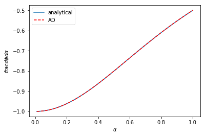
Now, we can plot the derivatives. I will plot both the analytical and automatic differentiated results.

%matplotlib inline
import matplotlib.pyplot as plt

# results from AD
alpha = np.linspace(0.01, 1)

# The AD derivative function is not vectorized, so we use this list comprehension.
dphidalpha = [adphi(a) for a in alpha]

def analytical_dphi(alpha):
    return -1 / (1 + alpha**2)

plt.plot(alpha, analytical_dphi(alpha), label='analytical')
plt.plot(alpha, dphidalpha, 'r--', label='AD')
plt.xlabel(r'$\alpha$')
plt.ylabel(r'$frac{d\phi}{d\alpha}$')
plt.legend()

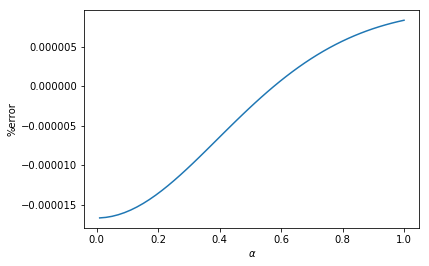
Visually, these are indistinguishable from each other. We can look at the errors too, and here we see they are negligible, and probably we can attribute them to the approximation we use for the integral, and not due to automatic differentiation.

perr = (analytical_dphi(alpha) - dphidalpha) / analytical_dphi(alpha) * 100
plt.plot(alpha, perr, label='analytical')
plt.xlabel(r'$\alpha$')
plt.ylabel('%error')

2 Example 2

In example 2 there is this function, which has variable limits:

\(f(x) = \int_{\sin x}^{\cos x} \cosh t^2 dt\)

What is \(f'(x)\) here? It can be derived with some effort and it is:

\(f'(x) = -\cosh(\cos^2 x) \sin x - \cosh(\sin^2 x) \cos x\)

This function was kind of fun to code up, I hadn't thought about how to represent variable limits, but here it is.

def f(x):
    a = np.sin(x)
    b = np.cos(x)
    t = np.linspace(a, b, 1000)
    y = np.cosh(t**2)
    return trapz(y, t)

# Here is our derivative!
dfdx = grad(f, 0)

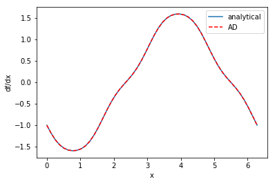
Here is a graphical comparison of the two:

x = np.linspace(0, 2 * np.pi)

analytical = -np.cosh(np.cos(x)**2) * np.sin(x) - \
    np.cosh(np.sin(x)**2) * np.cos(x)
ad = [dfdx(_x) for _x in x]

plt.plot(x, analytical, label='analytical')
plt.plot(x, ad, 'r--', label='AD')
plt.xlabel('x')
plt.ylabel('df/dx')
plt.legend()

These are once again indistinguishable.

3 Summary

These are amazing results to me. Before trying it, I would not have thought it would be so easy to evaluate the derivative of these functions. These work of course because all the operations involved in computing the integral are differentiable and defined in autograd. It certainly opens the door to all kinds of new approaches to solving engineering problems that need the derivatives for various purposes like optimization, sensitivity analysis, etc.

Copyright (C) 2018 by John Kitchin. See the License for information about copying.

org-mode source

Org-mode version = 9.1.13

Discuss on Twitter

Compressibility variation from an implicit equation of state

| categories: autograd, python | tags:

Table of Contents

In this post I explored using automatic differentiation to compute how the compressibility of a gas defined by the van der Waal equation varies with the reduced pressure. In that example we had an explicit function of the pressure as a function of the volume and temperature, and we could derive a differential equation that defines the variation we were interested in.

I thought we should be able to derive the differential equation more directly, still using automatic differentiation and we explore that idea here. The general strategy to compute the compressibility as a function of pressure is to integrate \(dV / dP_r\) over a range of \(P_r\) to get the molar volume as a function of \(P_r\), and then to directly compute the compressibility from \(Z = PV/(RT)\).

To use this approach we need to get \(dV / dP_r\) from the van der Waal equation. Previously, we derived this in a round about way from the explicit form of the van der Waal equation. Here, we follow the work in this post to get the derivative from the implicit form of the van der Waal equation:

\(f(V, P_r, T_r) = \frac{R Tr * Tc}{V - b} - \frac{a}{V^2} - P_r Pc = 0\)

Based on the work in this post, we can get

\(dV/dP_r = (-df/dP_r) / (df/dV)\)

and the two derivatives on the right can be found easily by automatic differentiation. First, we express the van der Waal equation in implicit form, with the variables as \(V, P_r, T_r\). Only two of those variables are independent; if you define two of them you can compute the third one using a tool like fsolve.

R = 0.08206
Pc = 72.9
Tc = 304.2

a = 27 * R**2 * Tc**2 / (Pc * 64)
b = R * Tc / (8 * Pc)

Tr = 1.1  # Constant for this example

def f(V, Pr, Tr):
    return R * Tr * Tc / (V - b) - a / V**2 - Pr * Pc

Now, if we want to know how does the volume vary with \(P_r\), we need to derive the derivative \(dV/dP_r\), and then integrate it. Here we use autograd to define the derivatives, and then we define a function that uses them. Note the arguments in the function dVdPr are in an order that anticipates we want to integrate it in solve_ivp, to get a function \(V(P_r)\).

from autograd import grad

dfdPr = grad(f, 1)  # derivative of f with respect to arg at index=1: Pr
dfdV = grad(f, 0)  # derivative of f with respect to arg at index=0: V

def dVdPr(Pr, V):
    return -dfdPr(V, Pr, Tr) / dfdV(V, Pr, Tr)  # Tr is a constant in here

Now, we need an initial condition to start the integration from. We want the volume at \(P_r=0.1\). We have to use fsolve for this, or some other method that tells you want is the volume at \(P_r=0.1\). We can pass the values of \(P_r\) and \(T_R\) as arguments to our implicit function. Since \(V\) is the first argument, we can directly solve our implicit function. Otherwise you would have to define a helper objective function to use with fsolve.

from scipy.optimize import fsolve

V0, = fsolve(f, 3.5, args=(0.1, 1.1))
V0
3.6764763125625435

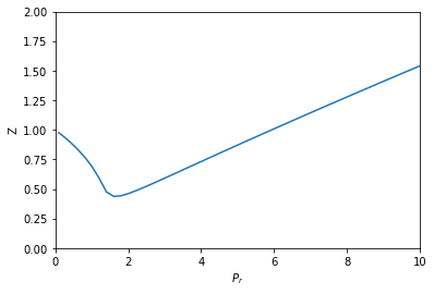
Finally, we are ready to integrate the ODE, and plot the solution.

import numpy as np
from scipy.integrate import solve_ivp

Pr_span = (0.1, 10)
Pr_eval, h = np.linspace(*Pr_span, retstep=True)

sol = solve_ivp(dVdPr, Pr_span, (V0,), max_step=h)
print(sol.message)

%matplotlib inline
import matplotlib.pyplot as plt

Pr = sol.t  # the P_r steps used in the solution
V = sol.y[0]  # V(P_r) from the solution

Z = Pr * Pc * V / (R * Tr * Tc)  # Compressibility Z(P_r)

plt.plot(Pr, Z)
plt.xlabel('$P_r$')
plt.ylabel('Z')
plt.xlim([0, 10])
plt.ylim([0, 2])
The solver successfully reached the end of the integration interval.


(0, 2)

That is the same result as we got before.

1 Summary thoughts

This method also worked successfully to solve this problem. In most ways, this method has less algebraic manipulations required to get to the solution. In method 3, we had to do some calculus that relied on a particular explicit form of the van der Waal equation. While those manipulations were not particularly difficulty, the leave opportunities for mistakes, and they will be more difficult for an implicit equation of state (e.g. if there was a \(P\) on the right hand side).

This approach also required some manipulation, but it is a standard one and that is how do you get a derivative from an implicit function. After that, it is straightforward to define the desired derivative as a function and then integrate it to get the solution. So, we still don't get a free pass on calculus, but we do reduce the number of manipulations required to get to the solution. I consider that a plus.

Copyright (C) 2018 by John Kitchin. See the License for information about copying.

org-mode source

Org-mode version = 9.1.13

Discuss on Twitter

Getting derivatives from implicit functions with autograd

| categories: autograd, python | tags:

If we have an implicit function: \(f(x, y(x)) = 0\), but we want to compute the derivative \(dy/dx\) we can use the chain rule to derive:

\(df/dx + df/dy dy/dx = 0\)

We can then solve for \(dy/dx\):

\(dy/dx = -df/dx / df/dy\) to get the desired derivative. The interesting point of this blog post is that we can get the two derivatives on the right hand side of this equation using automatic differentiation of the function \(f(x, y)\)! There are a few examples of analytical approaches to derivatives from implicit functions here, and I wanted to explore them with autograd in this post.

In the following examples, we will assume that \(y\) is a function of \(x\) and that \(x\) is independent. We will consider a series of implicit equations, compute \(dy/dx\) using autograd from the formula above, and compare them to the analytical results in the web page referenced above.

The \(dy/dx\) functions generally depend on both \(x\), and \(y\). Technically, these are the derivatives along the curve \(y(x)\), but since we can evaluate them at any points, we will use some random points for \(x\) and \(y\) to test for equality between the analytical derivatives and the autograd derivatives. This isn't a rigorous proof of equality, but it is the only thing that makes sense to do for now. It is assumed that if these points are ok, all the others are too. That might be a broad claim, since we only sample \(x\) and \(y\) from 0 to 1 here but the approach is general. Here are the imports and the random test points for all the examples that follow.

import autograd.numpy as np
from autograd import grad

xr = np.random.random(50)
yr = np.random.random(50)

1 Example 1

\(x^3 + y^3 = 4\)

def f1(x, y):
    return x**3 + y**3 - 4

D1x = grad(f1, 0)
D1y = grad(f1, 1)

dydx_1 = lambda x, y: -D1x(x, y) / D1y(x, y)
dydx_1a = lambda x, y: -x**2 / y**2

np.allclose(dydx_1a(xr, yr),
             [dydx_1(_xr, _yr) for _xr, _yr in zip(xr, yr)])
True

The output of True means the autograd results and the analytical results are "all close", i.e. within a tolerance the results are the same. The required derivatives of this are not that difficult to derive, but it is nice to see a simple example that "just works". A subtle point of the dydx function is that it is not vectorized which is why I used a list comprehension to evaluate all the points. It might be possible to make a pseudo-vectorized version with the np.vectorize decorator, but that is not of interest here.

2 Example 2

\((x - y)^2 = x + y - 1\)

def f2(x, y):
    return (x - y)**2 - x - y + 1

D2x = grad(f2, 0)
D2y = grad(f2, 1)

dydx_2 = lambda x, y: -D2x(x, y) / D2y(x, y)
dydx2_a = lambda x, y: (2 * y - 2 * x + 1) / (2 * y - 2 * x - 1)

np.allclose(dydx2_a(xr, yr),
            [dydx_2(_xr, _yr) for _xr, _yr in zip(xr, yr)])
True

This also works.

3 Example 3

\(y = sin(3x + 4y)\)

def f3(x, y):
    return y - np.sin(3 * x + 4 * y)


D3x = grad(f3, 0)
D3y = grad(f3, 1)

dydx_3 = lambda x, y: -D3x(x, y) / D3y(x, y)
dydx3_a = lambda x, y: (3 * np.cos(3 * x + 4 * y)) / (1 - 4 * np.cos(3 * x + 4 * y))

np.allclose(dydx3_a(xr, yr),
            [dydx_3(_xr, _yr) for _xr, _yr in zip(xr, yr)])
True

Check.

4 Example 4

\(y = x^2 y^3 + x^3 y^2\)

def f4(x, y):
    return y - x**2 * y**3 - x**3 * y**2


D4x = grad(f4, 0)
D4y = grad(f4, 1)

dydx_4 = lambda x, y: -D4x(x, y) / D4y(x, y)
dydx4_a = lambda x, y: (2 * x * y**3 + 3 * x**2 * y**2) / (1 - 3 * x**2 * y**2 - 2 * x**3 * y)

np.allclose(dydx4_a(xr, yr),
            [dydx_4(_xr, _yr) for _xr, _yr in zip(xr, yr)])
True

5 Example 5

\(e^{xy} = e^{4x} - e^{5y}\)

def f5(x, y):
    return np.exp(4 * x) - np.exp(5 * y) - np.exp(x * y)

D5x = grad(f5, 0)
D5y = grad(f5, 1)

dydx_5 = lambda x, y: -D5x(x, y) / D5y(x, y)
dydx5_a = lambda x, y: (4 * np.exp(4 * x) - y * np.exp(x * y)) / (x * np.exp(x * y) + 5 * np.exp(5 * y))

np.allclose(dydx5_a(xr, yr),
            [dydx_5(_xr, _yr) for _xr, _yr in zip(xr, yr)])
True

Also check.

6 Example 6

\(\cos^2 x + cos^2 y = cos(2x + 2y)\)

def f6(x, y):
    return np.cos(x)**2 + np.cos(y)**2 - np.cos(2 * x + 2 * y)

D6x = grad(f6, 0)
D6y = grad(f6, 1)

dydx_6 = lambda x, y: -D6x(x, y) / D6y(x, y)
dydx6_a = lambda x, y: (np.cos(x) * np.sin(x) - np.sin(2 * x + 2 * y)) / (np.sin(2 * x + 2 * y) - np.cos(y) * np.sin(y))

np.allclose(dydx6_a(xr, yr),
            [dydx_6(_xr, _yr) for _xr, _yr in zip(xr, yr)])
True

Check.

7 Example 7

\(x = 3 + \sqrt{x^2 + y^2}\)

def f7(x, y):
    return 3 + np.sqrt(x**2 + y**2) - x

D7x = grad(f7, 0)
D7y = grad(f7, 1)

dydx_7 = lambda x, y: -D7x(x, y) / D7y(x, y)
dydx7_a = lambda x, y: (np.sqrt(x**2 + y**2) - x) / y

np.allclose(dydx7_a(xr, yr),
            [dydx_7(_xr, _yr) for _xr, _yr in zip(xr, yr)])
True

8 Conclusions

There are a handful of other examples at the website referenced in the beginning, but I am stopping here. After seven examples of quantitative agreement between the easy to derive autograd derivatives, and the easy to moderately difficult analytical derivatives, it seems like it is autograd for the win here. This technique has some important implications for engineering calculations that I will explore in a future post. Until then, this is yet another interesting thing we can do with automatic differentiation!

Copyright (C) 2018 by John Kitchin. See the License for information about copying.

org-mode source

Org-mode version = 9.1.13

Discuss on Twitter
Next Page ยป