Using autograd to plot implicit functions

| categories: autograd, nonlinear-algebra, implicit-function | tags:

Consider the solution to these equations (adapted from https://www.mathworks.com/help/optim/ug/fsolve.html):

\(e^{-e^{-(x_1 + x_2)}} = x_2 (1 + x_1^2)\)

and

\(x_1 \cos(x_2) + x_2 \sin(x_1) = 1/2\)

It is not clear how many solutions there are to this set of equations, or what you should guess for the initial guess. Usually, the best way to see where a solution might be is to plot the equations and see where they intersect. These equations are implicit though, and it is not easy to plot them because we cannot solve for \(x_2\) in terms of \(x_1\) in either case. Here we explore a strategy to get plots so we can see where solutions could be.

The idea is that we find one solution to each equation independently. Then, we derive a differential equation for each equation so we can integrate it to find the curve that is defined by the implicit function. First, we find a solution for each equation. We guess a value for \(x_2\) and then find the value of \(x_1\) that solves each equation independently.

import autograd.numpy as np
from scipy.optimize import fsolve

def f1(x1, x2):
    return np.exp(-np.exp(-(x1 + x2))) - x2 * (1 + x1**2)

def f2(x1, x2):
    return x1 * np.cos(x2) + x2 * np.sin(x1) - 0.5

x2_1 = 0.6
x1_1, = fsolve(f1, 0, args=(x2_1,))
print('f1: ', x1_1, x2_1)

x2_2 = 1.0
x1_2, = fsolve(f2, 0 ,args=(x2_2,))
print('f2: ', x1_2, x2_2)

f1: 0.08638978040861575 0.6 f2: 0.32842406163614396 1.0

Next, we need a differential equation that is \(dx_2/dx_1\). If we had that, we could just integrate it from one of the starting points above, and get the curve we want. The functions are implicit, so we have to use the implicit derivative, which for the first equation is \(dx_2/dx_1 = -df1/dx_1 / df1/dx_2\). We will get these gradients from autograd. Then, we just integrate the solution. Here we do this for the first equation.

from scipy.integrate import solve_ivp
from autograd import grad

df1dx1 = grad(f1, 0)
df1dx2 = grad(f1, 1)

def dx2dx1_1(x1, x2):
    return -df1dx1(x1, x2) / df1dx2(x1, x2)

x1_span = (x1_1, 1)
x2_0 = (x2_1, )
sol1 = solve_ivp(dx2dx1_1, x1_span, x2_0, max_step=0.1)

And then, we do it for the second equation.

df2dx1 = grad(f2, 0)
df2dx2 = grad(f2, 1)

def dx2dx1_2(x1, x2):
    return -df2dx1(x1, x2) / df2dx2(x1, x2)

x1_span = (x1_2, 1)
x2_0 = (x2_2, )
sol2 = solve_ivp(dx2dx1_2, x1_span, x2_0, max_step=0.1)

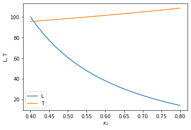
Finally, we plot the two solutions.

%matplotlib inline
import matplotlib.pyplot as plt
plt.plot(sol1.t, sol1.y.T)
plt.plot(sol2.t, sol2.y.T)
plt.xlabel('$x_1$')
plt.ylabel('$x_2$')
plt.legend(['f1', 'f2'])
<Figure size 432x288 with 1 Axes>

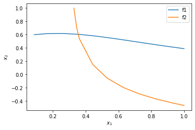
You can see now that in this range, there is only one intersection, i.e. one solution, and it is near \(x_1=0.4, x_2=0.6\). We can finally use that as an initial guess to find the only solution in this region, with confidence we are not missing any solutions.

def objective(X):
    x1, x2 = X
    return [f1(x1, x2), f2(x1, x2)]

fsolve(objective, [0.4, 0.6])
array([0.35324662, 0.60608174])

That is the same solution as reported at the Matlab site. Another use of autograd for the win here.

Copyright (C) 2019 by John Kitchin. See the License for information about copying.

org-mode source

Org-mode version = 9.2.3

Discuss on Twitter

Solving differential algebraic equations with help from autograd

| categories: autograd, dae, ode | tags:

This problem is adapted from one in "Problem Solving in Chemical Engineering with Numerical Methods, Michael B. Cutlip, Mordechai Shacham".

In the binary, batch distillation of benzene (1) and toluene (2), the moles of liquid \(L\) remaining as a function of the mole fraction of toluene (\(x_2\)) is expressed by:

\(\frac{dL}{dx_2} = \frac{L}{x_2 (k_2 - 1)}\)

where \(k_2\) is the vapor liquid equilibrium ratio for toluene. This can be computed as:

\(k_i = P_i / P\) where \(P_i = 10^{A_i + \frac{B_i}{T +C_i}}\) and that pressure is in mmHg, and the temperature is in degrees Celsius.

One difficulty in solving this problem is that the temperature is not constant; it changes with the composition. We know that the temperature changes to satisfy this constraint \(k_1(T) x_1 + k_2(T) x_2 = 1\).

Sometimes, one can solve for T directly, and substitute it into the first ODE, but this is not a possibility here. One way you might solve this is to use the constraint to find \(T\) inside an ODE function, but that is tricky; nonlinear algebra solvers need a guess and don't always converge, or may converge to non-physical solutions. They also require iterative solutions, so they will be slower than an approach where we just have to integrate the solution. A better way is to derive a second ODE \(dT/dx_2\) from the constraint. The constraint is implicit in \(T\), so We compute it as \(dT/dx_2 = -df/dx_2 / df/dT\) where \(f(x_2, T) = k_1(T) x_1 + k_2(T) x_2 - 1 = 0\). This equation is used to compute the bubble point temperature. Note, it is possible to derive these analytically, but who wants to? We can use autograd to get those derivatives for us instead.

The following information is given:

The total pressure is fixed at 1.2 atm, and the distillation starts at \(x_2=0.4\). There are initially 100 moles in the distillation.

species A B C
benzene 6.90565 -1211.033 220.79
toluene 6.95464 -1344.8 219.482

We have to start by finding the initial temperature from the constraint.

import autograd.numpy as np
from autograd import grad
from scipy.integrate import solve_ivp
from scipy.optimize import fsolve
%matplotlib inline
import matplotlib.pyplot as plt

P = 760 * 1.2 # mmHg
A1, B1, C1 = 6.90565, -1211.033,  220.79
A2, B2, C2 = 6.95464, -1344.8, 219.482

def k1(T):
    return 10**(A1 + B1 / (C1 + T)) / P

def k2(T):
    return 10**(A2 + B2 / (C2 + T)) / P

def f(x2, T):
    x1 = 1 - x2
    return k1(T) * x1 + k2(T) * x2 - 1

T0, = fsolve(lambda T: f(0.4, T), 96)
print(f'The initial temperature is {T0:1.2f} degC.')

The initial temperature is 95.59 degC.

Next, we compute the derivative we need. This derivative is derived from the constraint, which should ensure that the temperature changes as required to maintain the constraint.

dfdx2 = grad(f, 0)
dfdT = grad(f, 1)

def dTdx2(x2, T):
    return -dfdx2(x2, T) / dfdT(x2, T)

def ode(x2, X):
    L, T = X
    dLdx2 = L / (x2 * (k2(T) - 1))
    return [dLdx2, dTdx2(x2, T)]

Next we solve and plot the ODE.

x2span = (0.4, 0.8)
X0 = (100, T0)
sol = solve_ivp(ode, x2span, X0, max_step=0.01)

plt.plot(sol.t, sol.y.T)
plt.legend(['L', 'T']);
plt.xlabel('$x_2$')
plt.ylabel('L, T')
x2 = sol.t
L, T = sol.y
print(f'At x2={x2[-1]:1.2f} there are {L[-1]:1.2f} moles of liquid left at {T[-1]:1.2f} degC')

At x2=0.80 there are 14.04 moles of liquid left at 108.57 degC

<Figure size 432x288 with 1 Axes>

You can see that the liquid level drops, and the temperature rises.

Let's double check that the constraint is actually met. We do that qualitatively here by plotting it, and quantitatively by showing all values are close to 0.

constraint = k1(T) * (1 - x2) + k2(T) * x2 - 1
plt.plot(x2, constraint)
plt.ylim([-1, 1])
plt.xlabel('$x_2$')
plt.ylabel('constraint value')
print(np.allclose(constraint, np.zeros_like(constraint)))
constraint

True

array([ 2.22044605e-16,  4.44089210e-16,  2.22044605e-16,  0.00000000e+00,
        1.11022302e-15,  0.00000000e+00,  6.66133815e-16,  0.00000000e+00,
       -2.22044605e-16,  1.33226763e-15,  8.88178420e-16, -4.44089210e-16,
        4.44089210e-16,  1.11022302e-15, -2.22044605e-16,  0.00000000e+00,
       -2.22044605e-16, -1.11022302e-15,  4.44089210e-16,  0.00000000e+00,
       -4.44089210e-16,  4.44089210e-16, -6.66133815e-16, -4.44089210e-16,
        4.44089210e-16, -1.11022302e-16, -8.88178420e-16, -8.88178420e-16,
       -9.99200722e-16, -3.33066907e-16, -7.77156117e-16, -2.22044605e-16,
       -9.99200722e-16, -1.11022302e-15, -3.33066907e-16, -1.99840144e-15,
       -1.33226763e-15, -2.44249065e-15, -1.55431223e-15, -6.66133815e-16,
       -2.22044605e-16])
<Figure size 432x288 with 1 Axes>

So indeed, the constraint is met! Once again, autograd comes to the rescue in making a computable derivative from an algebraic constraint so that we can solve a DAE as a set of ODEs using our regular machinery. Nice work autograd!

Copyright (C) 2019 by John Kitchin. See the License for information about copying.

org-mode source

Org-mode version = 9.2.3

Discuss on Twitter

Sensitivity analysis with odeint and autograd

| categories: autograd, ode | tags:

In this previous post I showed a way to do sensitivity analysis of the solution of a differential equation to parameters in the equation using autograd. The basic approach was to write a differentiable integrator, and then use it in a function so that autograd could take the derivative.

Since that time, autograd has added derivative support for scipy.integrate.odeint. In this post we examine that. As usual with autograd, we have to import the autograd version of numpy, and the autograd version of odeint. We will find the derivative of the solution to an ODE (which is an array) so we need to also import the jacobian function. Finally, there is a subtle, and non-obvious requirement that we need to import the autograd tuple. That ensures that the variables are differentiable through the tuple we will use for the arguments.

The differential equation we solve returns the concentration of a species as a function of time, and the solution depends on two parameters, i.e. \(C = f(t; k_1, k_{-1})\), and we are interested in the time-dependent sensitivity of \(C\) with respect to those parameters. The approach we use is to define a function that has those parameters as arguments. The function will solve the ODE and return the time-dependent solution. First we make that solution, mostly to see that the autograd version of odeint works.

import autograd.numpy as np
from autograd.scipy.integrate import odeint
from autograd import jacobian
from autograd.builtins import tuple

import matplotlib.pyplot as plt

Ca0 = 1.0
k1 = k_1 = 3.0

tspan = np.linspace(0, 0.5)

def C(K):
    k1, k_1 = K
    def dCdt(Ca, t, k1, k_1):
        return -k1 * Ca + k_1 * (Ca0 - Ca)
    sol = odeint(dCdt, Ca0, tspan, tuple((k1, k_1)))
    return sol

plt.plot(tspan, C([k1, k_1]))
plt.xlim([tspan.min(), tspan.max()])
plt.xlabel('t')
plt.ylabel('C');
<Figure size 432x288 with 1 Axes>

Now, the solution is an array, and we want the derivative of C with respect to the parameters at each time point. That means we want the jacobian derivative of the output with respect to the input. Here is the autograd approach to doing that. The jacobian function returns a function that we can evaluate to get the derivatives.

import time
t0 = time.time()
dCdk = jacobian(C, 0)


k_sensitivity = dCdk(np.array([k1, k_1]))

k1_sensitivity = k_sensitivity[:, 0, 0]
k_1_sensitivity = k_sensitivity[:, 0, 1]

plt.plot(tspan, np.abs(k1_sensitivity), label='dC/dk1')
plt.plot(tspan, np.abs(k_1_sensitivity), label='dC/dk_1')
plt.legend(loc='best')
plt.xlabel('t')
plt.ylabel('sensitivity')
print(f'Elapsed time = {time.time() - t0:1.1f} seconds')

Elapsed time = 38.2 seconds

<Figure size 432x288 with 1 Axes>

That looks similar to the results from before. It is pretty slow I think, that took more than half a minute to work out. That is still faster and probably more correct than if I had to do it by hand. In contrast, however, the finite difference code below is comparatively very fast! I don't know what is slow in the autograd implementation. I guess it is an implementation detail.

import numdifftools as nd
t0 = time.time()

fdk1, fdk_1 = nd.Jacobian(C)([k1, k_1]).T
print(f'Elapsed time = {time.time() - t0:1.1f} seconds')

plt.plot(tspan, np.abs(fdk1), label='fd dC/dk1')
plt.plot(tspan, np.abs(fdk_1), label='fd dC/dk_1')
plt.plot(tspan, np.abs(k1_sensitivity), 'y--', label='dC/dk1')
plt.plot(tspan, np.abs(k_1_sensitivity),'m--', label='dC/dk_1')
plt.legend(loc='best');
plt.xlabel('t');
plt.ylabel('sensitivity');

Elapsed time = 0.1 seconds

<Figure size 432x288 with 1 Axes>

You can see the two results are visually indistinguishable. Even the code is pretty similar. I would tend to prefer the autograd way since it should be less sensitive to finite difference artifacts, but it is nice to have an independent way to test if it is working.

Copyright (C) 2019 by John Kitchin. See the License for information about copying.

org-mode source

Org-mode version = 9.2.3

Discuss on Twitter

Line integrals in Python with autograd

| categories: integration, autograd, python | tags:

Table of Contents

A line integral is an integral of a function along a curve in space. We usually represent the curve by a parametric equation, e.g. \(\mathbf{r}(t) = [x(t), y(t), z(t)] = x(t)\mathbf{i} + y(t)\mathbf{j} + z(t)\mathbf{k}\). So, in general the curve will be a vector function, and the function we want to integrate will also be a vector function.

Then, we can write the line integral definition as:

\(\int_C \mathbf{F(r)}\cdot d\mathbf{r} = \int_a^b \mathbf{F}({\mathbf{r}(t)) \cdot \mathbf{r'}(t) dt\) where \(\mathbf{r'}(t) = \frac{d\mathbf{r}}{dt}\). This integrand is a scalar function, because of the dot product.

The following examples are adapted from Chapter 10 in Advanced Engineering Mathematics by Kreysig.

The first example is the evaluation of a line integral in the plane. We want to evaluate the integral of \(\mathbf{F(r)}=[-y, -xy]\) on the curve \(\mathbf{r(t)}=[-sin(t), cos(t)]\) from t=0 to t = π/2. The answer in the book is given as 0.4521. Here we evaluate this numerically, using autograd for the relevant derivative. Since the curve has multiple outputs, we have to use the jacobian function to get the derivatives. After that, it is a simple bit of matrix multiplication, and a call to the quad function.

import autograd.numpy as np
from autograd import jacobian
from scipy.integrate import quad

def F(X):
    x, y = X
    return -y, -x * y

def r(t):
    return np.array([-np.sin(t), np.cos(t)])

drdt = jacobian(r)

def integrand(t):
    return F(r(t)) @ drdt(t)

I, e = quad(integrand, 0.0, np.pi / 2)
print(f'The integral is {I:1.4f}.')
The integral is 0.4521.


We get the same result as the analytical solution.

The next example is in three dimensions. Find the line integral along \(\mathbf{r}(t)=[cos(t), sin(t), 3t]\) of the function \(\mathbf{F(r)}=[z, x, y]\) from t=0 to t=2 π. The solution is given as 21.99.

import autograd.numpy as np
from autograd import elementwise_grad, grad, jacobian

def F(X):
    x, y, z = X
    return [z, x, y]

def C(t):
    return np.array([np.cos(t), np.sin(t), 3 * t])

dCdt = jacobian(C, 0)

def integrand(t):
    return F(C(t)) @ dCdt(t)

I, e = quad(integrand, 0, 2 * np.pi)
print(f'The integral is {I:1.2f}.')
The integral is 21.99.


That is also the same as the analytical solution. Note the real analytical solution was 7 π, which is nearly equivalent to our answer.

7 * np.pi - I
3.552713678800501e-15

As a final example, we consider an alternate form of the line integral. In this form we do not use a dot product, so the integral results in a vector. This doesn't require anything from autograd, but does require us to be somewhat clever in how to do the integrals since quad can only integrate scalar functions. We need to integrate each component of the integrand independently. Here is one approach where we use lambda functions for each component. You could also manually separate the components.

def F(r):
    x, y, z = r
    return x * y, y * z, z

def r(t):
    return np.array([np.cos(t), np.sin(t), 3 * t])

def integrand(t):
    return F(r(t))

[quad(lambda t: integrand(t)[i], 0, 2 * np.pi)[0] for i in [0, 1, 2]]
[-6.9054847581172525e-18, -18.849555921538755, 59.21762640653615]

The analytical solution in this case was given as:

[0, -6 * np.pi, 6 * np.pi**2]
[0, -18.84955592153876, 59.21762640653615]

which is evidently the same as our numerical solution.

Maybe an alternative, but more verbose is this vectorized integrate function. We still make temporary functions for integrating, and the vectorization is essentially like the list comprehension above, but we avoid the lambda functions.

@np.vectorize
def integrate(i):
    def integrand(t):
        return F(r(t))[i]
    I, e = quad(integrand, 0, 2 * np.pi)
    return I

integrate([0, 1, 2])
array([ -6.90548476e-18,  -1.88495559e+01,   5.92176264e+01])

1 Summary

Once again, autograd provides a convenient way to compute function jacobians which make it easy to evaluate line integrals in Python.

Copyright (C) 2018 by John Kitchin. See the License for information about copying.

org-mode source

Org-mode version = 9.1.14

Discuss on Twitter

Using autograd for error propagation

| categories: autograd, uncertainty | tags:

Back in 2013 I wrote about using the uncertainties package to propagate uncertainties. The problem setup was for finding the uncertainty in the exit concentration from a CSTR when there are uncertainties in the other parameters. In this problem we were given this information about the parameters and their uncertainties.

Parameter value σ
Fa0 5 0.05
v0 10 0.1
V 66000 100
k 3 0.2

The exit concentration is found by solving this equation:

\(0 = Fa0 - v0 * Ca - k * Ca**2 * V\)

So the question was what is Ca, and what is the uncertainty on it? Finding Ca is easy with fsolve.

from scipy.optimize import fsolve

Fa0 = 5.0
v0 = 10.0

V = 66000.0
k = 3.0

def func(Ca, v0, k, Fa0, V):
    "Mole balance for a CSTR. Solve this equation for func(Ca)=0"
    Fa = v0 * Ca     # exit molar flow of A
    ra = -k * Ca**2  # rate of reaction of A L/mol/h
    return Fa0 - Fa + V * ra

Ca, = fsolve(func, 0.1 * Fa0 / v0, args=(v0, k, Fa0, V))
Ca
0.0050000000000000001

The uncertainty on Ca is a little trickier. A simplified way to estimate it is:

\(\sigma_{Ca} = \sqrt{(dCa/dv0)^2 \sigma_{v0}^2 + (dCa/dv0)^2 \sigma_{v0}^2 + (dCa/dFa0)^2 \sigma_{Fa0}^2 + (dCa/dV)^2 \sigma_{V}^2}\)

We know the σ_i for each input, we just need those partial derivatives. However, we only have the implicit function we used to solve for Ca, and I do not want to do the algebra to solve for Ca. Luckily, we previously worked out how to get these derivatives from an implicit function using autograd. We just need to loop through the arguments, get the relevant derivatives, and accumulate the product of the squared derivatives and errors. Finally, take the square root of that sum.

import autograd.numpy as np
from autograd import grad

# these are the uncertainties on the inputs
s = [None, 0.1, 0.2, 0.05, 100]

S2 = 0.0

dfdCa = grad(func, 0)
for i in range(1, 5):
    dfdarg2 = grad(func, i)
    dCadarg2 = -dfdarg2(Ca, v0, k, Fa0, V) / dfdCa(Ca, v0, k, Fa0, V)
    S2 += dCadarg2**2 * s[i]**2

Ca_s = np.sqrt(S2)
print(f'Ca = {Ca:1.5f} +\- {Ca_s}')
Ca = 0.00500 +\- 0.00016776432898276802


That is the same uncertainty estimate the quantities package provided. One benefit here is I did not have to do the somewhat complicated wrapping procedure around fsolve that was required with uncertainties to get this. On the other hand, I did have to derive the formula and implement them. It worked fine here, since we have an implicit function and a way to get the required derivatives. It could take some work to do this with the exit concentration of a PFR, which requires an integrator. Maybe that differentiable integrator will come in handy again!

Copyright (C) 2018 by John Kitchin. See the License for information about copying.

org-mode source

Org-mode version = 9.1.14

Discuss on Twitter
Next Page ยป