The Kitchin Research Group

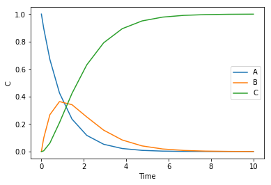
Here is the standard numerical solution to this problem. This will give us a reference for what the solution should look like.

from scipy.integrate import solve_ivp

def ode(t, C):
    Ca, Cb, Cc = C
    dCadt = -k1 * Ca
    dCbdt = k1 * Ca - k2 * Cb
    dCcdt = k2 * Cb
    return [dCadt, dCbdt, dCcdt]

C0 = [1.0, 0.0, 0.0]
k1 = 1
k2 = 1

sol = solve_ivp(ode, (0, 10), C0)

%matplotlib inline
import matplotlib.pyplot as plt

plt.plot(sol.t, sol.y.T)
plt.legend(['A', 'B', 'C'])
plt.xlabel('Time')
plt.ylabel('C')

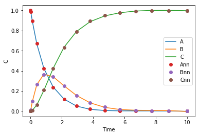
The first thing I want to show is that you can train a neural network to reproduce this solution. That is certainly a prerequisite to the idea working. We use the same code I used before, but this time our neural network will output three values, one for each concentration.

import autograd.numpy as np
from autograd import grad, elementwise_grad, jacobian
import autograd.numpy.random as npr
from autograd.misc.optimizers import adam

def init_random_params(scale, layer_sizes, rs=npr.RandomState(0)):
    """Build a list of (weights, biases) tuples, one for each layer."""
    return [(rs.randn(insize, outsize) * scale,   # weight matrix
             rs.randn(outsize) * scale)           # bias vector
            for insize, outsize in zip(layer_sizes[:-1], layer_sizes[1:])]

def swish(x):
    "see https://arxiv.org/pdf/1710.05941.pdf"
    return x / (1.0 + np.exp(-x))

def C(params, inputs):
    "Neural network functions"
    for W, b in params:
        outputs = np.dot(inputs, W) + b
        inputs = swish(outputs)
    return outputs

# initial guess for the weights and biases
params = init_random_params(0.1, layer_sizes=[1, 8, 3])

Now, we train our network to reproduce the solution. I ran this block manually a bunch of times, but eventually you see that we can train a one layer network with 8 nodes to output all three concentrations pretty accurately. So, there is no issue there, a neural network can represent the solution.

def objective_soln(params, step):
    return np.sum((sol.y.T - C(params, sol.t.reshape([-1, 1])))**2)

params = adam(grad(objective_soln), params,
              step_size=0.001, num_iters=500)

plt.plot(sol.t.reshape([-1, 1]), C(params, sol.t.reshape([-1, 1])),
         sol.t, sol.y.T, 'o')
plt.legend(['A', 'B', 'C', 'Ann', 'Bnn', 'Cnn'])
plt.xlabel('Time')
plt.ylabel('C')

The next issue is how do we get the relevant derivatives. The solution method I developed here relies on using optimization to find a set of weights that produces a neural network whose derivatives are consistent with the ODE equations. So, we need to be able to get the derivatives that are relevant in the equations.

The neural network outputs three concentrations, and we need the time derivatives of them. Autograd provides three options: grad, elementwise_grad and jacobian. We cannot use grad because our function is not scalar. We cannot use elementwise_grad because that will give the wrong shape (I think it may be the sum of the gradients). That leaves us with the jacobian. This, however, gives an initially unintuitive (i.e. it isn't what we need out of the box) result. The output is 4-dimensional in this case, consistent with the documentation of that function.

jacC = jacobian(C, 1)
jacC(params, sol.t.reshape([-1, 1])).shape

(17, 3, 17, 1)

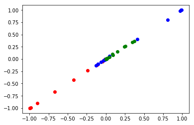
Why does it have this shape? Our time input vector we used has 17 time values, in a column vector. That leads to an output from the NN with a shape of (17, 3), i.e. the concentrations of each species at each time. The jacobian will output an array of shape (17, 3, 17, 1), and we have to extract the pieces we want from that. The first and third dimensions are related to the time steps. The second dimension is the species, and the last dimension is nothing here, but is there because the input is in a column. I use some fancy indexing on the array to get the desired arrays of the derivatives. This is not obvious out of the box. I only figured this out by direct comparison of the data from a numerical solution and the output of the jacobian. Here I show how to do that, and make sure that the derivatives we pull out are comparable to the derivatives defined by the ODEs above. Parity here means they are comparable.

i = np.arange(len(sol.t))
plt.plot(jacC(params, sol.t.reshape([-1, 1]))[i, 0, i, 0],   -k1 * sol.y[0], 'ro')
plt.plot(jacC(params, sol.t.reshape([-1, 1]))[i, 1, i, 0],   -k2 * sol.y[1] + k1 * sol.y[0], 'bo')
plt.plot(jacC(params, sol.t.reshape([-1, 1]))[i, 2, i, 0],   k2 * sol.y[1], 'go')

[<matplotlib.lines.Line2D at 0x118a2e860>]

Note this is pretty inefficient. It requires a lot of calculations (the jacobian here has print(17*3*17) 867 elements) to create the jacobian, and we don't need most of them. You could avoid this by creating separate neural networks for each species, and then just use elementwise_grad on each one. Alternatively, one might be able to more efficiently compute some vector-jacobian product. Nevertheless, it looks like we can get the correct derivatives out of the neural network, we just need a convenient function to return them. Here is one such function for this problem, using a fancier slicing and reshaping to get the derivative array.

# Derivatives
jac = jacobian(C, 1)

def dCdt(params, t):
    i = np.arange(len(t))
    return jac(params, t)[i, :, i].reshape((len(t), 3))

Finally, we are ready to try solving the ODEs solely by the neural network approach. We reinitialize the neural network first, and define a time grid to solve it on.

t = np.linspace(0, 10, 25).reshape((-1, 1))
params = init_random_params(0.1, layer_sizes=[1, 8, 3])
i = 0    # number of training steps
N = 501  # epochs for training
et = 0.0 # total elapsed time

We define our objective function. This function will be zero at the perfect solution, and has contributions for each mole balance and the initial conditions. It could make sense to put additional penalties for things like negative concentrations, or the sum of concentrations is a constant, but we do not do that here, and it does not seem to be necessary.

def objective(params, step):
    Ca, Cb, Cc = C(params, t).T
    dCadt, dCbdt, dCcdt = dCdt(params, t).T

    z1 = np.sum((dCadt + k1 * Ca)**2)
    z2 = np.sum((dCbdt - k1 * Ca + k2 * Cb)**2)
    z3 = np.sum((dCcdt - k2 * Cb)**2)
    ic = np.sum((np.array([Ca[0], Cb[0], Cc[0]]) - C0)**2)  # initial conditions
    return z1 + z2 + z3 + ic

def callback(params, step, g):
    if step % 100 == 0:
        print("Iteration {0:3d} objective {1}".format(step,
                                                      objective(params, step)))

objective(params, 0)  # make sure the objective is scalar

5.2502237371050295

Finally, we run the optimization. I also manually ran this block several times.

import time
t0 = time.time()

params = adam(grad(objective), params,
              step_size=0.001, num_iters=N, callback=callback)

i += N
t1 = (time.time() - t0) / 60
et += t1

plt.plot(t, C(params, t), sol.t, sol.y.T, 'o')
plt.legend(['Ann', 'Bnn', 'Cnn', 'A', 'B', 'C'])
plt.xlabel('Time')
plt.ylabel('C')
print(f'{t1:1.1f} minutes elapsed this time. Total time = {et:1.2f} min. Total epochs = {i}.')

Iteration   0 objective 0.00047651643957525214
Iteration 100 objective 0.0004473301532609342
Iteration 200 objective 0.00041218410058863227
Iteration 300 objective 0.00037161526137030344
Iteration 400 objective 0.000327567400443358
Iteration 500 objective 0.0002836975879675981
0.6 minutes elapsed this time. Total time = 4.05 min. Total epochs = 3006.

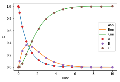
The effort seems to have been worth it though, we get a pretty good solution from our neural network.

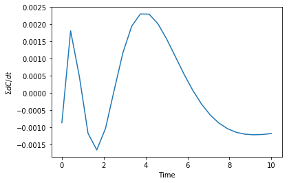
We can check the accuracy of the derivatives by noting the sum of the derivatives in this case should be zero. Here you can see that the sum is pretty small. It would take additional optimization to a lower error to get this to be smaller.

plt.plot(t, np.sum(dCdt(params, t), axis=1))
plt.xlabel('Time')
plt.ylabel(r'$\Sigma dC/dt$')

In the end, this method is illustrated to work for systems of ODEs also. There is some subtlety in how to get the relevant derivatives from the jacobian, but after that, it is essentially the same. I think it would be much faster to do this with separate neural networks for each function in the solution because then you do not need the jacobian, you can use elementwise_grad.

This is not faster than direct numerical integration. One benefit to this solution over a numerical solution is we get an actual continuous function as the solution, rather than an array of data. This solution is not reliable at longer times, but then again neither is extrapolation of numeric data. It could be interesting to explore if this has any benefits for stiff equations. Maybe another day. For now, I am declaring victory for autograd on this problem.