The Kitchin Research Group

In the last post I explored using a neural network to solve a BVP. Here, I expand the idea to solving an initial value ordinary differential equation. The idea is basically the same, we just have a slightly different objective function.

\(dCa/dt = -k Ca(t)\) where \(Ca(t=0) = 2.0\).

Here is the code that solves this equation, along with a comparison to the analytical solution: \(Ca(t) = Ca0 \exp -kt\).

import autograd.numpy as np
from autograd import grad, elementwise_grad
import autograd.numpy.random as npr
from autograd.misc.optimizers import adam

def init_random_params(scale, layer_sizes, rs=npr.RandomState(0)):
    """Build a list of (weights, biases) tuples, one for each layer."""
    return [(rs.randn(insize, outsize) * scale,   # weight matrix
             rs.randn(outsize) * scale)           # bias vector
            for insize, outsize in zip(layer_sizes[:-1], layer_sizes[1:])]


def swish(x):
    "see https://arxiv.org/pdf/1710.05941.pdf"
    return x / (1.0 + np.exp(-x))


def Ca(params, inputs):
    "Neural network functions"
    for W, b in params:
        outputs = np.dot(inputs, W) + b
        inputs = swish(outputs)    
    return outputs

    
# Here is our initial guess of params:
params = init_random_params(0.1, layer_sizes=[1, 8, 1])

# Derivatives
dCadt = elementwise_grad(Ca, 1)

k = 0.23
Ca0 = 2.0
t = np.linspace(0, 10).reshape((-1, 1))

# This is the function we seek to minimize
def objective(params, step):
    # These should all be zero at the solution
    # dCadt = -k * Ca(t)
    zeq = dCadt(params, t) - (-k * Ca(params, t))
    ic = Ca(params, 0) - Ca0
    return np.mean(zeq**2) + ic**2

def callback(params, step, g):
    if step % 1000 == 0:
        print("Iteration {0:3d} objective {1}".format(step,
                                                      objective(params, step)))

params = adam(grad(objective), params,
              step_size=0.001, num_iters=5001, callback=callback) 


tfit = np.linspace(0, 20).reshape(-1, 1)
import matplotlib.pyplot as plt
plt.plot(tfit, Ca(params, tfit), label='soln')
plt.plot(tfit, Ca0 * np.exp(-k * tfit), 'r--', label='analytical soln')
plt.legend()
plt.xlabel('time')
plt.ylabel('$C_A$')
plt.xlim([0, 20])
plt.savefig('nn-ode.png')

Iteration   0 objective [[ 3.20374053]]
Iteration 1000 objective [[  3.13906829e-05]]
Iteration 2000 objective [[  1.95894699e-05]]
Iteration 3000 objective [[  1.60381564e-05]]
Iteration 4000 objective [[  1.39930673e-05]]
Iteration 5000 objective [[  1.03554970e-05]]

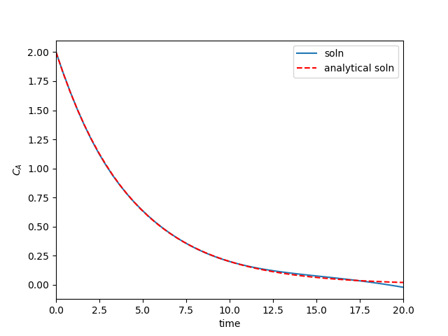
Huh. Those two solutions are nearly indistinguishable. Since we used a neural network, let's hype it up and say we learned the solution to a differential equation! But seriously, note that although we got an "analytical" solution, we should only rely on it in the region we trained the solution on. You can see the solution above is not that good past t=10, even perhaps going negative (which is not even physically correct). That is a reminder that the function we have for the solution is not the same as the analytical solution, it just approximates it really well over the region we solved over. Of course, you can expand that region to the region you care about, but the main point is don't rely on the solution outside where you know it is good.

This idea isn't new. There are several papers in the literature on using neural networks to solve differential equations, e.g. http://www.sciencedirect.com/science/article/pii/S0255270102002076 and https://arxiv.org/pdf/physics/9705023.pdf, and other blog posts that are similar (https://becominghuman.ai/neural-networks-for-solving-differential-equations-fa230ac5e04c, even using autograd). That means to me that there is some merit to continuing to investigate this approach to solving differential equations.

There are some interesting challenges for engineers to consider with this approach though. When is the solution accurate enough? How reliable are derivatives of the solution? What network architecture is appropriate or best? How do you know how good the solution is? Is it possible to build in solution features, e.g. asymptotes, or constraints on derivatives, or that the solution should be monotonic, etc. These would help us trust the solutions not to do weird things, and to extrapolate more reliably.

Copyright (C) 2017 by John Kitchin. See the License for information about copying.

org-mode source

Org-mode version = 9.1.2