Batch / Parallel Design of Experiments#
When experimental capacity is parallel (several reactors, wells, or
robots that run together), designing experiments one at a time wastes
information. This tutorial demonstrates discopt.doe.batch_optimal_experiment,
which selects \(N\) experimental conditions jointly under D/A/E/ME
optimality.
Mathematical background. For independent experiments the Fisher information matrix is additive,
and the joint D-optimal batch maximises \(\log\det \text{FIM}_{\text{total}}\) over the stacked design vector \((d_1, \dots, d_N)\). This formulation follows Galvanin et al. [2007]; we also support a cheaper greedy strategy (pick one, fold into the prior, repeat) and a distance-penalized variant. For robust / expected-information variants the reader is referred to Sandrin et al. [2025]. For an alternative route via parallel Bayesian optimization rather than FIM-based MBDoE, see González and Zavala [2023].
import os

os.environ.setdefault("JAX_PLATFORMS", "cpu")
os.environ.setdefault("JAX_ENABLE_X64", "1")

import discopt.modeling as dm
import numpy as np
from discopt.doe import (
    BatchStrategy,
    DesignCriterion,
    batch_optimal_experiment,
    sequential_doe,
)
from discopt.estimate import Experiment, ExperimentModel, estimate_parameters
Toy experiment#
A first-order decay \(y = A \exp(-k t)\) with one design variable (sampling time \(t\)) and one unknown parameter (\(k\)).
class ExpDecay(Experiment):
    def create_model(self, **kwargs):
        m = dm.Model("expdecay")
        k = m.continuous("k", lb=0.01, ub=5)
        t = m.continuous("t", lb=0.1, ub=10)
        return ExperimentModel(
            model=m,
            unknown_parameters={"k": k},
            design_inputs={"t": t},
            responses={"y": 5.0 * dm.exp(-k * t)},
            measurement_error={"y": 0.05},
        )


exp = ExpDecay()
param_values = {"k": 0.5}
bounds = {"t": (0.1, 10.0)}
Greedy batch#
Pick one design, fold its FIM into the running prior, repeat. Cheap and
incremental, and it reuses the single-design optimal_experiment search.
greedy = batch_optimal_experiment(
    exp,
    param_values=param_values,
    design_bounds=bounds,
    n_experiments=4,
    strategy=BatchStrategy.GREEDY,
    criterion=DesignCriterion.D_OPTIMAL,
)
print(greedy.summary())
print()
print("per-round criterion:", greedy.per_round_criterion)
Batch Optimal Design (N=4, strategy=greedy)
============================================================
  Experiment 1:
                  t = 2
  Experiment 2:
                  t = 2
  Experiment 3:
                  t = 1.99996
  Experiment 4:
                  t = 2.00002

  D-opt (log det joint FIM) = 9.983
  A-opt (trace joint FIM⁻¹) = 4.618e-05
  E-opt (min eigenval)      = 2.165e+04
  Condition number          = 1

  SE(k) = 0.006796

per-round criterion: [8.59663473309607, 9.289781913656014, 9.695247021621437, 9.982929094074354]
Joint batch (Galvanina-style)#
Stack the \(N\) design vectors and optimize them simultaneously with scipy L-BFGS-B over the joint criterion. Slower than greedy on nonlinear experiments but equal or better in information content. The formulation follows Galvanin et al. [2007].
joint = batch_optimal_experiment(
    exp,
    param_values=param_values,
    design_bounds=bounds,
    n_experiments=4,
    strategy=BatchStrategy.JOINT,
    criterion=DesignCriterion.D_OPTIMAL,
)
print(joint.summary())
print()
print(f"greedy log det FIM = {greedy.criterion_value:.4g}")
print(f"joint  log det FIM = {joint.criterion_value:.4g}")
Batch Optimal Design (N=4, strategy=joint)
============================================================
  Experiment 1:
                  t = 1.99995
  Experiment 2:
                  t = 1.99997
  Experiment 3:
                  t = 2.00001
  Experiment 4:
                  t = 2.00001

  D-opt (log det joint FIM) = 9.983
  A-opt (trace joint FIM⁻¹) = 4.618e-05
  E-opt (min eigenval)      = 2.165e+04
  Condition number          = 1

  SE(k) = 0.006796

greedy log det FIM = 9.983
joint  log det FIM = 9.983
Penalized batch#
Greedy with a normalized min-distance filter: useful when you want spatial diversity across the batch (e.g. to avoid clustering probes even if the criterion is locally indifferent).
penalized = batch_optimal_experiment(
    exp,
    param_values=param_values,
    design_bounds=bounds,
    n_experiments=4,
    strategy=BatchStrategy.PENALIZED,
    criterion=DesignCriterion.D_OPTIMAL,
    min_distance=0.15,
)
print(penalized.summary())
Batch Optimal Design (N=4, strategy=penalized)
============================================================
  Experiment 1:
                  t = 2
  Experiment 2:
                  t = 4.25778
  Experiment 3:
                  t = 6.20369
  Experiment 4:
                  t = 7.81546

  D-opt (log det joint FIM) = 9.105
  A-opt (trace joint FIM⁻¹) = 0.0001111
  E-opt (min eigenval)      = 9004
  Condition number          = 1

  SE(k) = 0.01054
Sequential batch MBDoE#
sequential_doe(experiments_per_round=N, batch_strategy=...) alternates
parameter estimation and batch design, which is the pattern typically
deployed in an automated laboratory. Each round designs \(N\) experiments
jointly and the runner callback is invoked once per batch member.
The loop merges whatever the runner returns into the cumulative data
by response key, and estimate_parameters reads repeated values under
one key as replicates at the model’s fixed conditions — the design
values are not attached to the data. So a runner that always returns
{"y": value} throws away the very thing the design step chose: every
observation is fitted at one condition and \(\hat{k}\) never converges.
(sequential_doe warns when it sees this.)
The pattern that works is a stateful experiment: each observation collected so far becomes its own response at its own fixed time, and only the next slot carries the design variable \(t\). The runner appends the new observation to that state and returns it under a fresh key.
class AccumulatingExpDecay(Experiment):
    """Same decay, but the model grows with the data.

    ``observations`` holds one ``(label, t)`` pair per datum gathered so
    far; each becomes a response at its own *fixed* time. A single extra
    response, ``y_next``, carries the design variable, so that is what
    the batch designer varies.
    """

    def __init__(self):
        self.observations: list[tuple[str, float]] = []

    def add_observation(self, label: str, t: float) -> None:
        self.observations.append((label, float(t)))

    def create_model(self, **kwargs):
        m = dm.Model("expdecay_sequential")
        k = m.continuous("k", lb=0.01, ub=5)
        responses = {label: 5.0 * dm.exp(-k * t) for label, t in self.observations}
        t_var = m.continuous("t", lb=0.1, ub=10)
        responses["y_next"] = 5.0 * dm.exp(-k * t_var)
        return ExperimentModel(
            model=m,
            unknown_parameters={"k": k},
            design_inputs={"t": t_var},
            responses=responses,
            measurement_error={name: 0.05 for name in responses},
        )


k_true = 0.7
rng = np.random.default_rng(0)


def measure(t):
    return float(5.0 * np.exp(-k_true * t) + rng.normal(0.0, 0.05))


seq_exp = AccumulatingExpDecay()
initial_data = {}
for i, t0 in enumerate([0.5, 2.0]):
    label = f"y_init_{i}"
    seq_exp.add_observation(label, t0)
    initial_data[label] = measure(t0)

collected = {"n": 0}


def runner(design):
    collected["n"] += 1
    label = f"y_round_{collected['n']}"
    t = float(design["t"])
    seq_exp.add_observation(label, t)
    return {label: measure(t)}


history = sequential_doe(
    seq_exp,
    initial_data=initial_data,
    initial_guess={"k": 0.5},
    design_bounds=bounds,
    n_rounds=3,
    experiments_per_round=2,
    batch_strategy=BatchStrategy.GREEDY,
    run_experiment=runner,
)
for r in history:
    ts = [round(d["t"], 3) for d in r.design.designs]
    print(f"round {r.round}: k_hat = {r.estimation.parameters['k']:.3f}, batch t = {ts}")
round 0: k_hat = 0.701, batch t = [1.427, 1.427]
round 1: k_hat = 0.696, batch t = [1.437, 1.437]
round 2: k_hat = 0.698, batch t = [1.432, 1.432]
Each round estimates before collecting its own data, so the last
k_hat above is one round stale. Refit on everything to close the loop.
all_data = dict(initial_data)
for r in history:
    all_data.update(r.data_collected)

final = estimate_parameters(
    seq_exp, all_data, initial_guess=history[-1].estimation.parameters
)
print(f"{len(all_data)} observations")
print(f"final k_hat = {final.parameters['k']:.3f}   (k_true = {k_true})")
No valid dual bound was produced for model 'expdecay_sequential': the relaxation layer could not bound this objective (status=feasible). The result cannot be certified globally optimal. A nonlinear term with no envelope is the usual cause; an epigraph reformulation (minimize z subject to f(x) <= z) often gives the relaxation something to bound.
8 observations
final k_hat = 0.693   (k_true = 0.7)
Notes and scope#
What is supported: joint D/A/E/ME optimality over \(N\) independent
experiments with continuous design bounds, with an additive prior
FIM carried forward by sequential_doe.
What is out of scope in v1:
Robust / expected-information designs \(\mathbb{E}_\theta[\text{FIM}]\) under parameter uncertainty (see Sandrin et al. [2025] for a modern framework).
Mixed-integer batch designs (choose \(N\) from a discrete candidate pool).
Bayesian-style q-acquisitions on GP surrogates; for that flavour of parallel experiment design see González and Zavala [2023].
Heterogeneous batches (different
Experimenttypes in one batch).End-to-end JAX autograd through the joint objective; the joint solver currently uses scipy finite differences.