Identifiability and Estimability Analysis

Identifiability and Estimability Analysis#

This notebook demonstrates the three identifiability diagnostics added in response to issue #45:

diagnose_identifiability — Belsley/Kuh/Welsch regression diagnostics plus the Gutenkunst sloppy-model eigenvalue spectrum [Belsley et al., 1980, Gutenkunst et al., 2007].
estimability_rank — Yao-style orthogonalization ranking with the Brun collinearity index on top of discopt’s existing compute_fim Jacobian [Brun et al., 2001, Yao et al., 2003].
profile_likelihood — Raue/Kreutz profile-likelihood confidence intervals and shape classification [Kreutz et al., 2013, Raue et al., 2009].

The worked example is a four-parameter series reaction kinetics model where two rate constants enter only as their product, producing a classic practical non-identifiability. We use this to demonstrate each diagnostic and show that they agree on which direction is non-identifiable [Miao et al., 2011, Villaverde, 2019].

Reparameterization note. The Yao ranking and the Belsley condition indices are not invariant under a change of variable such as \(\theta \to \log \theta\). Profile likelihood is invariant. If a diagnostic flags non-identifiability, try a log-reparameterization before concluding the parameter itself is at fault.

import os

os.environ.setdefault("JAX_PLATFORMS", "cpu")
os.environ.setdefault("JAX_ENABLE_X64", "1")
# The fit below is deliberately non-identifiable, so the solver logs a
# progress note on every iteration of every profile. Interesting once,
# thousands of lines by the end of the notebook.
os.environ.setdefault("RUST_LOG", "warn")

import warnings

import discopt.modeling as dm
import matplotlib.pyplot as plt
import numpy as np
from discopt.doe import (
    diagnose_identifiability,
    estimability_rank,
    profile_all,
    profile_likelihood,
)
from discopt.estimate import Experiment, ExperimentModel, estimate_parameters

# A singular FIM means negative variances, so the standard errors come back
# nan. That is the finding, not an error -- the summary tables show it.
warnings.filterwarnings(
    "ignore", category=RuntimeWarning, message="invalid value encountered in sqrt"
)

np.random.seed(42)

The model#

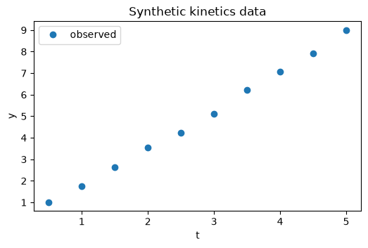
Series first-order reactions \(A \xrightarrow{k_1} B \xrightarrow{k_2} C\) observed at a set of time points, with an additional constant baseline and a quadratic nuisance term.

We build the response as

\[y(t) = \alpha \cdot k_1 \cdot k_2 \cdot t + c_0 + c_2 t^2\]

so that:

The product \(k_1 k_2\) (and \(\alpha\)) appears linearly through the single combined parameter \(\alpha k_1 k_2\); only two of \(\{\alpha, k_1, k_2\}\) are algebraically identifiable.
\(c_0\) and \(c_2\) are fully identifiable on their own.

This is the canonical “practical non-identifiability by overparameterization” scenario [Yao et al., 2003].

class KineticsExperiment(Experiment):
    def __init__(self, t_data):
        self.t_data = t_data

    def create_model(self, **kwargs):
        m = dm.Model("kinetics")
        alpha = m.continuous("alpha", lb=0.1, ub=5.0)
        k1 = m.continuous("k1", lb=0.01, ub=5.0)
        k2 = m.continuous("k2", lb=0.01, ub=5.0)
        c0 = m.continuous("c0", lb=-5.0, ub=5.0)
        c2 = m.continuous("c2", lb=-1.0, ub=1.0)

        responses = {}
        errors = {}
        for i, t in enumerate(self.t_data):
            responses[f"y_{i}"] = alpha * k1 * k2 * t + c0 + c2 * t * t
            errors[f"y_{i}"] = 0.1

        return ExperimentModel(
            m,
            unknown_parameters={"alpha": alpha, "k1": k1, "k2": k2, "c0": c0, "c2": c2},
            design_inputs={},
            responses=responses,
            measurement_error=errors,
        )


# True parameter values (note: alpha*k1*k2 = 1.5)
alpha_true = 1.0
k1_true = 1.5
k2_true = 1.0
c0_true = 0.2
c2_true = 0.05

t_data = np.linspace(0.5, 5.0, 10)
exp = KineticsExperiment(t_data)

# Generate synthetic data with Gaussian noise.
data = {}
for i, t in enumerate(t_data):
    mu = alpha_true * k1_true * k2_true * t + c0_true + c2_true * t * t
    data[f"y_{i}"] = mu + np.random.normal(0, 0.1)

fig, ax = plt.subplots(figsize=(6, 3.5))
ax.plot(t_data, [data[f"y_{i}"] for i in range(len(t_data))], "o", label="observed")
ax.set_xlabel("t")
ax.set_ylabel("y")
ax.set_title("Synthetic kinetics data")
ax.legend()

<matplotlib.legend.Legend at 0x111aecbc0>

../_images/9a2f94fa88ee2e0ec9a9834482a8a495f2ef5fdc07b4fbbcc083243c3fca3009.png

Step 1 — Fit the full model#

Use estimate_parameters to obtain maximum-likelihood estimates \(\hat{\theta}\) and the deviance \(D(\hat{\theta})\) at the optimum.

est = estimate_parameters(
    exp,
    data,
    initial_guess={
        "alpha": alpha_true,
        "k1": k1_true,
        "k2": k2_true,
        "c0": c0_true,
        "c2": c2_true,
    },
)
print(est.summary())

Duals withheld (#1037): the backend's multipliers violate complementary slackness against the box your model declares at alpha.lb(declared 0.1, CS 9.091e-06), k1.lb(declared 0.01, CS 9.091e-06), k2.lb(declared 0.01, CS 9.091e-06), c0.lb(declared -5, CS 9.091e-06), c2.lb(declared -1, CS 9.091e-06) …, so they are duals of a different problem. Refitting against the declared active set did not reach stationarity (residual 1.748e-04 > 1.000e-06), so no duals are reported rather than wrong ones.

No valid dual bound was produced for model 'kinetics': the relaxation layer could not bound this objective (status=feasible). The result cannot be certified globally optimal. A nonlinear term with no envelope is the usual cause; an epigraph reformulation (minimize z subject to f(x) <= z) often gives the relaxation something to bound.

Parameter Estimation Results
==================================================
         alpha =      1.32939  ± nan  [nan, nan]
            k1 =      1.07298  ± nan  [nan, nan]
            k2 =      1.07298  ± nan  [nan, nan]
            c0 =     0.216697  ± 0.1176  [-0.08564, 0.519]
            c2 =    0.0441992  ± 0.01741  [-0.0005489, 0.08895]
     Objective = 4.5897
         N obs = 10
       FIM det = 4.516e-14
      FIM cond = 1.229e+17

Note that the point estimates of \(\alpha\), \(k_1\), \(k_2\) will not agree with the true values — because only their product is identifiable, the optimizer picks some triple lying on the ridge \(\alpha k_1 k_2 = 1.5\).

Step 2 — Diagnose identifiability#

diagnose_identifiability returns the full Belsley/Gutenkunst diagnostic bundle. The condition indices, variance-inflation factors, variance-decomposition proportions, and the log-eigenvalue spectrum all point at the same offending direction [Belsley et al., 1980, Gutenkunst et al., 2007].

diag = diagnose_identifiability(exp, est.parameters)
print(f"FIM rank: {diag.fim_rank}/{diag.n_parameters}")
print(f"Condition number: {diag.condition_number:.3g}")
print()
print("Condition indices:", np.round(diag.condition_indices, 3))
print()
print("VIFs:")
for name, v in diag.vif.items():
    print(f"  {name:>6s}: {v:.3g}")
print()
print("Warnings:")
for w in diag.warnings:
    print(" ", w)

FIM rank: 3/5
Condition number: 1.55e+17

Condition indices: [1.00000000e+00 4.34900000e+00 2.04860000e+01 2.54295104e+16
 5.86866216e+16]

VIFs:
   alpha: inf
      k1: inf
      k2: inf
      c0: 2.16
      c2: 2.16

Warnings:
  mild collinearity: condition index eta_3 = 20.5 > 10
  serious collinearity: condition index eta_4 = 2.54e+16 > 30
  serious collinearity: condition index eta_5 = 5.87e+16 > 30
  VIF[alpha] is infinite (parameter lies in a null direction)
  VIF[k1] is infinite (parameter lies in a null direction)
  VIF[k2] is infinite (parameter lies in a null direction)
  |rho[k1,k2]| = 1.41e+07 > 0.95
  |rho[k1,c0]| = 1.24 > 0.95
  |rho[k1,c2]| = 1.19 > 0.95

# Sloppy-model spectrum (Gutenkunst)
fig, (ax1, ax2) = plt.subplots(1, 2, figsize=(10, 3.5))
ax1.plot(np.arange(1, len(diag.normalized_log_spectrum) + 1), diag.normalized_log_spectrum, "o-")
ax1.set_xlabel("eigenvalue index (descending)")
ax1.set_ylabel(r"$\log_{10}(\lambda / \lambda_\max)$")
ax1.set_title("FIM eigenvalue spectrum")
ax1.axhline(-6, color="red", linestyle="--", alpha=0.3, label="sloppy (-6 decades)")
ax1.legend()

# VIF bar chart
names = list(diag.vif.keys())
vifs = [diag.vif[n] for n in names]
vifs_plot = [min(v, 1e3) for v in vifs]
ax2.bar(names, vifs_plot, color=["red" if np.isinf(v) or v > 10 else "steelblue" for v in vifs])
ax2.axhline(10, color="black", linestyle="--", alpha=0.4, label="VIF=10")
ax2.set_ylabel("VIF (clipped at 1e3)")
ax2.set_title("Variance Inflation Factors")
ax2.set_yscale("log")
ax2.legend()
plt.tight_layout()

../_images/cb275da54fff6b7d8d91783f90e8ca9493efef6eae62cdb8bdc973e0fcc23074.png

The parameter \(k_2\) and \(k_1\) show infinite VIFs (or large finite ones depending on the fit), and the log-eigenvalue spectrum spans multiple decades — the classic sloppy signature.

Inspect the null-space direction directly:

if diag.null_space:
    print("Null direction(s) in (normalized) parameter space:")
    for d in diag.null_space:
        for name, coef in d.items():
            print(f"  {name:>6s}: {coef:+.4f}")
else:
    print("FIM is full rank (no strict null direction at this tolerance).")

Null direction(s) in (normalized) parameter space:
   alpha: +0.7243
      k1: -0.6885
      k2: -0.0358
      c0: -0.0000
      c2: -0.0000
   alpha: -0.3768
      k1: -0.4389
      k2: +0.8157
      c0: +0.0000
      c2: +0.0000

Step 3 — Estimability ranking (Yao / Brun)#

estimability_rank ranks parameters from most to least estimable using rank-revealing QR on the Brun-scaled sensitivity matrix [Yao et al., 2003]. The projected 2-norm at step \(k\) equals \(|R_{kk}|\) from the QR and matches Yao’s paper numerically.

rank = estimability_rank(exp, est.parameters)
print("Ranking (most -> least estimable):")
for name, pn in zip(rank.ranking, rank.projected_norms):
    bar = "=" * max(1, int(50 * pn / max(rank.projected_norms[0], 1e-30)))
    print(f"  {name:>6s}  |R_kk| = {pn:10.4g}  {bar}")
print()
print(f"Recommended subset at cutoff 0.04: {rank.recommended_subset}")
print(f"Collinearity index of the recommended subset: {rank.collinearity_index:.3g}")

Ranking (most -> least estimable):
      k2  |R_kk| =      150.2  ==================================================
      c2  |R_kk| =      4.372  =
      c0  |R_kk| =      1.842  =
      k1  |R_kk| =  3.643e-14  =
   alpha  |R_kk| =  9.694e-15  =

Recommended subset at cutoff 0.04: ['k2']
Collinearity index of the recommended subset: 1

Step 4 — Profile likelihood#

profile_likelihood steps \(\theta_i\) outward from the estimate in both directions, re-optimizing all other parameters at each step, and records the deviance \(D(\theta)\). The 95% confidence region is \(\{\theta_i : D(\theta_i) - D(\hat\theta) \le \chi^2_{1, 0.95}\}\) (deviance convention — no factor of 1/2, see module docstring) [Kreutz et al., 2013, Raue et al., 2009].

profile_all re-optimizes at every step of every profile, and each of those fits repeats the “duals withheld” warning you saw in Step 1 — the model is singular, so the solver declines to report multipliers it cannot certify. Correct, and identical 55 times over. It is a logging record from discopt.solver, so quiet it there.

import contextlib
import logging


@contextlib.contextmanager
def quiet_solver():
    """Drop `discopt.solver` warnings for the duration of the block."""
    log = logging.getLogger("discopt.solver")
    previous = log.level
    log.setLevel(logging.ERROR)
    try:
        yield
    finally:
        log.setLevel(previous)

with quiet_solver():
    profiles = profile_all(exp, data, confidence_level=0.95, max_steps=15)

for name, p in profiles.items():
    ci_lo = f"{p.ci_lower:.3g}" if p.ci_lower is not None else "-inf"
    ci_hi = f"{p.ci_upper:.3g}" if p.ci_upper is not None else "+inf"
    print(f"  {name:>6s}  shape={p.shape:17s}  95% CI = [{ci_lo}, {ci_hi}]")
    for w in p.warnings:
        print(f"          warn: {w}")

   alpha  shape=flat               95% CI = [-inf, +inf]
          warn: profile is flat: |D(theta) - D(theta_hat)| stays below 0.384; parameter is not practically identifiable
      k1  shape=one_sided_lower    95% CI = [0.804, +inf]
          warn: upper arm hit parameter bound ub=5 without crossing the threshold
      k2  shape=one_sided_lower    95% CI = [0.804, +inf]
          warn: upper arm hit parameter bound ub=5 without crossing the threshold
      c0  shape=flat               95% CI = [-inf, +inf]
          warn: neither arm crossed the threshold; parameter may be practically non-identifiable
      c2  shape=flat               95% CI = [-inf, +inf]
          warn: neither arm crossed the threshold; parameter may be practically non-identifiable

# Plot profiles for each parameter.
fig, axes = plt.subplots(1, len(profiles), figsize=(3 * len(profiles), 3.5), sharey=True)
for ax, (name, p) in zip(axes, profiles.items()):
    ax.plot(p.theta_values, p.neg_log_lik - p.objective_hat, "o-", markersize=3)
    ax.axhline(
        p.threshold - p.objective_hat, color="red", linestyle="--", label=r"$\chi^2_{1,0.95}$"
    )
    ax.axvline(p.theta_hat, color="black", linestyle=":", alpha=0.5)
    ax.set_title(f"{name}  ({p.shape})")
    ax.set_xlabel(r"$\theta$")
axes[0].set_ylabel(r"$D(\theta) - D(\hat\theta)$")
axes[0].legend()
plt.tight_layout()

Round-trip consistency#

All three diagnostics should identify the same non-identifiable direction:

diagnose_identifiability reports FIM rank < \(n_\text{params}\).
estimability_rank puts the redundant parameter last with a projected norm \(\approx 0\).
profile_likelihood shows a flat or one-sided profile for that parameter.

This pipeline-level agreement is what makes the tools trustworthy; if one flags a problem, the others should too [Villaverde, 2019].

non_identifiable = {p.parameter for p in profiles.values() if p.shape != "bounded"}
print("Parameters with non-bounded profile:", non_identifiable)

excluded = set(est.parameter_names) - set(rank.recommended_subset)
print("Parameters excluded by Yao ranking:", excluded)

null_param = set()
for d in diag.null_space:
    null_param |= {n for n, c in d.items() if abs(c) > 0.1}
print("Parameters with weight in FIM null space:", null_param)

Parameters with non-bounded profile: {'k2', 'c0', 'c2', 'alpha', 'k1'}
Parameters excluded by Yao ranking: {'c0', 'k1', 'c2', 'alpha'}
Parameters with weight in FIM null space: {'k2', 'alpha', 'k1'}

Worked example 2 — Langmuir adsorption isotherm#

The Langmuir isotherm

\[q(c) = \frac{q_m K c}{1 + K c}\]

has two parameters: the saturation capacity \(q_m\) and the affinity \(K\). Their identifiability depends critically on the concentration grid:

In the linear regime (\(Kc \ll 1\)) the model collapses to \(q \approx q_m K c\), so only the product \(q_m K\) is identifiable and the FIM is rank-1.
In the saturated regime (\(Kc \gtrsim 1\)) the curvature exposes \(q_m\) and \(K\) separately and the FIM is full rank.

This is a textbook practical-identifiability case [Brun et al., 2001, Raue et al., 2009].

class LangmuirExperiment(Experiment):
    def __init__(self, c_data, sigma=0.05):
        self.c_data = list(c_data)
        self.sigma = float(sigma)

    def create_model(self, **kwargs):
        m = dm.Model("langmuir")
        qm = m.continuous("qm", lb=0.01, ub=20.0)
        K = m.continuous("K", lb=1e-4, ub=1e4)
        responses = {f"q_{i}": qm * K * c / (1.0 + K * c) for i, c in enumerate(self.c_data)}
        errors = {k: self.sigma for k in responses}
        return ExperimentModel(m, {"qm": qm, "K": K}, {}, responses, errors)


qm_true, K_true = 5.0, 1.0
c_sat = np.array([0.1, 0.3, 1.0, 3.0, 10.0])  # spans linear AND saturated regimes
c_lin = np.array([0.001, 0.002, 0.005, 0.01, 0.02])  # linear regime only

# Compare diagnostics in the two regimes (using true values as the
# nominal point so we are not chasing fit noise).
diag_sat = diagnose_identifiability(LangmuirExperiment(c_sat), {"qm": qm_true, "K": K_true})
diag_lin = diagnose_identifiability(LangmuirExperiment(c_lin), {"qm": qm_true, "K": K_true})

print(f"Saturated regime: rank={diag_sat.fim_rank}, cond={diag_sat.condition_number:.3g}")
print(f"  VIFs: {diag_sat.vif}")
print()
print(f"Linear regime:    rank={diag_lin.fim_rank}, cond={diag_lin.condition_number:.3g}")
print(f"  VIFs: {diag_lin.vif}")

Saturated regime: rank=2, cond=10.1
  VIFs: {'qm': 2.6581230148182944, 'K': 2.6581230148182944}

Linear regime:    rank=2, cond=1.06e+06
  VIFs: {'qm': 40325.376368355515, 'K': 40325.37636835549}

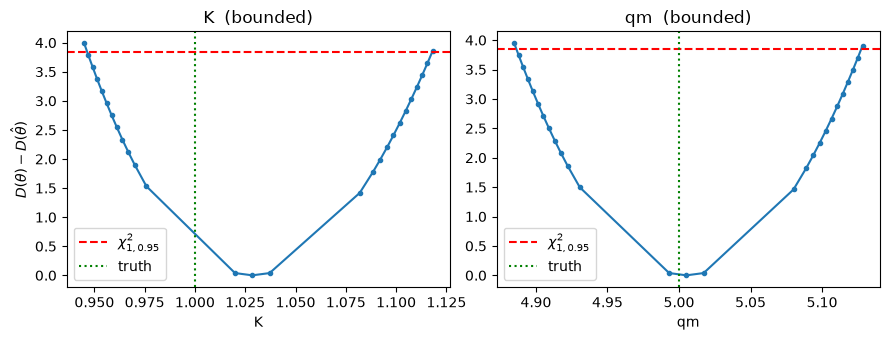
The linear regime exposes a near-singular FIM (condition number \(\gg 100\)) and inflated VIFs — the classic signature. Now profile likelihood the \(K\) parameter in the well-designed regime to confirm a bounded CI:

np.random.seed(42)
exp_sat = LangmuirExperiment(c_sat)
data_sat = {
    f"q_{i}": qm_true * K_true * c / (1 + K_true * c) + np.random.normal(0, 0.05)
    for i, c in enumerate(c_sat)
}
est_sat = estimate_parameters(exp_sat, data_sat, initial_guess={"qm": 4.0, "K": 0.5})
print(est_sat.summary())

prof_K = profile_likelihood(exp_sat, data_sat, "K", initial_estimate=est_sat)
prof_qm = profile_likelihood(exp_sat, data_sat, "qm", initial_estimate=est_sat)

fig, (a1, a2) = plt.subplots(1, 2, figsize=(9, 3.5))
for ax, p, name, true in [(a1, prof_K, "K", K_true), (a2, prof_qm, "qm", qm_true)]:
    ax.plot(p.theta_values, p.neg_log_lik - p.objective_hat, "o-", markersize=3)
    ax.axhline(p.threshold - p.objective_hat, color="red", ls="--", label=r"$\chi^2_{1,0.95}$")
    ax.axvline(true, color="green", ls=":", label="truth")
    ax.set_title(f"{name}  ({p.shape})")
    ax.set_xlabel(name)
    ax.legend()
a1.set_ylabel(r"$D(\theta) - D(\hat\theta)$")
plt.tight_layout()

No valid dual bound was produced for model 'langmuir': the relaxation layer could not bound this objective (status=feasible). The result cannot be certified globally optimal. A nonlinear term with no envelope is the usual cause; an epigraph reformulation (minimize z subject to f(x) <= z) often gives the relaxation something to bound.

Parameter Estimation Results
==================================================
            qm =      5.00517  ± 0.06176  [4.809, 5.202]
             K =       1.0285  ± 0.04408  [0.8882, 1.169]
     Objective = 1.6786
         N obs = 5
       FIM det = 3.546e+05
      FIM cond = 9.65

../_images/083f66bf307243d2ef6e3fe74ecbec8f13fa7adc3fe73246309c009a23923bfa.png

Worked example 3 — Batch reactor rate data#

A batch reactor obeying first-order kinetics with a non-zero asymptote:

\[C(t) = (C_0 - C_\infty) e^{-k t} + C_\infty\]

Three parameters: initial concentration \(C_0\), rate constant \(k\), and asymptote \(C_\infty\).

Whether all three are identifiable from a given experiment depends on how the time grid is chosen relative to the system’s relaxation time \(1/k\). If sampling stops before reaching the asymptote, \(C_\infty\) trades off with \(C_0\) and the FIM becomes ill-conditioned [Yao et al., 2003].

class BatchReactorExperiment(Experiment):
    def __init__(self, t_data, sigma=0.02):
        self.t_data = list(t_data)
        self.sigma = float(sigma)

    def create_model(self, **kwargs):
        m = dm.Model("batch_reactor")
        C0 = m.continuous("C0", lb=0.1, ub=10.0)
        k = m.continuous("k", lb=0.001, ub=10.0)
        C_inf = m.continuous("C_inf", lb=0.0, ub=5.0)
        responses = {
            f"C_{i}": (C0 - C_inf) * dm.exp(-k * t) + C_inf for i, t in enumerate(self.t_data)
        }
        errors = {kname: self.sigma for kname in responses}
        return ExperimentModel(m, {"C0": C0, "k": k, "C_inf": C_inf}, {}, responses, errors)


C0_true, k_true, Cinf_true = 5.0, 0.5, 1.0

# Long horizon: 5 half-lives -> all three identifiable.
t_long = np.linspace(0.0, 10.0, 11)
# Short horizon: < 1 half-life -> C_inf weakly identifiable.
t_short = np.linspace(0.0, 1.5, 8)

# Diagnose at the truth (no fitting noise).
diag_long = diagnose_identifiability(
    BatchReactorExperiment(t_long), {"C0": C0_true, "k": k_true, "C_inf": Cinf_true}
)
diag_short = diagnose_identifiability(
    BatchReactorExperiment(t_short), {"C0": C0_true, "k": k_true, "C_inf": Cinf_true}
)

print(f"Long horizon (t<=10):  rank={diag_long.fim_rank}/3, cond={diag_long.condition_number:.3g}")
print(f"  VIFs: {diag_long.vif}")
print(f"  warnings: {diag_long.warnings or '(none)'}")
print()
print(
    f"Short horizon (t<=1.5): rank={diag_short.fim_rank}/3, cond={diag_short.condition_number:.3g}"
)
print(f"  VIFs: {diag_short.vif}")
print("  warnings:")
for w in diag_short.warnings:
    print(f"    - {w}")

Long horizon (t<=10):  rank=3/3, cond=34.7
  VIFs: {'C0': 1.420210482619665, 'k': 2.9148440891797294, 'C_inf': 2.3045530043046623}
  warnings: (none)

Short horizon (t<=1.5): rank=3/3, cond=6.97e+03
  VIFs: {'C0': 3.264772067101546, 'k': 193.07215564199007, 'C_inf': 172.31260750258525}
  warnings:
    - serious collinearity: condition index eta_3 = 31.1 > 30
    - VIF[k] = 193 > 10
    - VIF[C_inf] = 172 > 10
    - |rho[k,C_inf]| = 0.994 > 0.95

The short-horizon design has a much larger condition number and one or more inflated VIFs — Yao’s ranking will recommend dropping the worst offender:

rank_short = estimability_rank(
    BatchReactorExperiment(t_short),
    {"C0": C0_true, "k": k_true, "C_inf": Cinf_true},
)
print("Yao ranking on the short-horizon experiment:")
top = rank_short.projected_norms[0]
for name, pn in zip(rank_short.ranking, rank_short.projected_norms):
    bar = "=" * max(1, int(40 * pn / max(top, 1e-30)))
    print(f"  {name:>6s}  |R_kk| = {pn:10.4g}  {bar}")
print()
print(f"Recommended subset (cutoff 0.04): {rank_short.recommended_subset}")
print(f"Collinearity index: {rank_short.collinearity_index:.3g}")

Yao ranking on the short-horizon experiment:
      C0  |R_kk| =      515.4  ========================================
       k  |R_kk| =      94.23  =======
   C_inf  |R_kk| =      3.653  =

Recommended subset (cutoff 0.04): ['C0', 'k']
Collinearity index: 2

Take-away. The three diagnostics (diagnose_identifiability \(\to\) condition number / VIF; estimability_rank \(\to\) projected norms; profile_likelihood \(\to\) shape) form a coherent picture: when the experiment’s design under-excites a parameter, all three flag it. A better-designed experiment (here, longer sampling horizon for the batch reactor; saturated-regime concentrations for Langmuir) restores identifiability. This is the model-based design-of-experiments loop in miniature [Villaverde, 2019].