Handling units with the quantities module

| categories: units | tags:

The quantities module (https://pypi.python.org/pypi/quantities) is another option for handling units in python. We are going to try the previous example. It does not work, because scipy.optimize.fsolve is not designed to work with units.

import quantities as u
import numpy as np

from scipy.optimize import fsolve
CA0 = 1 * u.mol / u.L
CA = 0.01 * u.mol / u.L
k = 1.0 / u.s

def func(t):
    return CA - CA0 * np.exp(-k * t)

tguess = 4 * u.s

print func(tguess)

print fsolve(func, tguess)
>>> >>> >>> >>> >>> >>> >>> ... ... >>> >>> >>> -0.00831563888873 mol/L
>>> Traceback (most recent call last):
  File "<stdin>", line 1, in <module>
  File "c:\Python27\lib\site-packages\scipy\optimize\minpack.py", line 115, in fsolve
    _check_func('fsolve', 'func', func, x0, args, n, (n,))
  File "c:\Python27\lib\site-packages\scipy\optimize\minpack.py", line 13, in _check_func
    res = atleast_1d(thefunc(*((x0[:numinputs],) + args)))
  File "<stdin>", line 2, in func
  File "c:\Python27\lib\site-packages\quantities-0.10.1-py2.7.egg\quantities\quantity.py", line 231, in __array_prepare__
    res._dimensionality = p_dict[uf](*objs)
  File "c:\Python27\lib\site-packages\quantities-0.10.1-py2.7.egg\quantities\dimensionality.py", line 347, in _d_dimensionless
    raise ValueError("quantity must be dimensionless")
ValueError: quantity must be dimensionless

Our function works fine with units, but fsolve does not pass numbers with units back to the function, so this function fails because the exponential function gets an argument with dimensions in it. We can create a new function that solves this problem. We need to “wrap” the function we want to solve to make sure that it uses units, but returns a float number. Then, we put the units back onto the final solved value. Here is how we do that.

import quantities as u
import numpy as np

from scipy.optimize import fsolve as _fsolve

CA0 = 1 * u.mol / u.L
CA = 0.01 * u.mol / u.L
k = 1.0 / u.s

def func(t):
    return CA - CA0 * np.exp(-k * t)

def fsolve(func, t0):
    'wrapped fsolve command to work with units'
    tU = t0 / float(t0)  # units on initial guess, normalized
    def wrapped_func(t):
        't will be unitless, so we add unit to it. t * tU has units.'
        return float(func(t * tU))

    sol, = _fsolve(wrapped_func, t0)
    return sol * tU
    
tguess = 4 * u.s

print fsolve(func, tguess)
4.60517018599 s

It is a little tedious to do this, but we might only have to do it once if we store the new fsolve command in a module. You might notice the wrapped function we wrote above only works for one dimensional problems. If there are multiple dimensions, we have to be a little more careful. In the next example, we expand the wrapped function definition to do both one and multidimensional problems. It appears we cannot use numpy.array element-wise multiplication because you cannot mix units in an array. We will use lists instead. When the problem is one-dimensional, the function will take a scalar, but when it is multidimensional it will take a list or array. We will use try/except blocks to handle these two cases. We will assume multidimensional cases, and if that raises an exception because the argument is not a list, we assume it is scalar. Here is the more robust code example.

import quantities as u
import numpy as np

from scipy.optimize import fsolve as _fsolve

def fsolve(func, t0):
    '''wrapped fsolve command to work with units. We get the units on
    the function argument, then wrap the function so we can add units
    to the argument and return floats. Finally we call the original
    fsolve from scipy. Note: this does not support all of the options
    to fsolve.''' 

    try:
        tU = [t / float(t) for t in t0]  # units on initial guess, normalized
    except TypeError:
        tU = t0 / float(t0)
    
    def wrapped_func(t):
        't will be unitless, so we add unit to it. t * tU has units.'    
        try:
            T = [x1 * x2 for x1,x2 in zip(t, tU)]
        except TypeError:
            T = t * tU

        try:
            return [float(x) for x in func(T)]
        except TypeError:
            return float(func(T))

    sol = _fsolve(wrapped_func, t0)
    try:
        return [x1 * x2 for x1,x2 in zip(sol, tU)]
    except TypeError:
        return sol * tU

### Problem 1
CA0 = 1 * u.mol / u.L
CA = 0.01 * u.mol / u.L
k = 1.0 / u.s

def func(t):
    return CA - CA0 * np.exp(-k * t)


tguess = 4 * u.s
sol1, = fsolve(func, tguess)
print 'sol1 = ',sol1

### Problem 2
def func2(X):
    a,b = X
    return [a**2 - 4*u.kg**2,
            b**2 - 25*u.J**2]

Xguess = [2.2*u.kg, 5.2*u.J]
s2a, s2b = fsolve(func2, Xguess)
print 's2a = {0}\ns2b = {1}'.format(s2a, s2b)
sol1 =  4.60517018599 s
s2a = 2.0 kg
s2b = 5.0 J

That is pretty good. There is still room for improvement in the wrapped function, as it does not support all of the options that scipy.optimize.fsolve supports. Here is a draft of a function that does that. We have to return different numbers of arguments depending on the value of full_output. This function works, but I have not fully tested all the options. Here are three examples that work, including one with an argument.

import quantities as u
import numpy as np

from scipy.optimize import fsolve as _fsolve

def fsolve(func, t0, args=(), 
           fprime=None, full_output=0, col_deriv=0, 
           xtol=1.49012e-08, maxfev=0, band=None, 
           epsfcn=0.0, factor=100, diag=None):
    '''wrapped fsolve command to work with units. We get the units on
    the function argument, then wrap the function so we can add units
    to the argument and return floats. Finally we call the original
    fsolve from scipy. ''' 

    try:
        tU = [t / float(t) for t in t0]  # units on initial guess, normalized
    except TypeError:
        tU = t0 / float(t0)
    
    def wrapped_func(t, *args):
        't will be unitless, so we add unit to it. t * tU has units.'    
        try:
            T = [x1 * x2 for x1,x2 in zip(t, tU)]
        except TypeError:
            T = t * tU

        try:
            return [float(x) for x in func(T, *args)]
        except TypeError:
            return float(func(T))

    sol = _fsolve(wrapped_func, t0, args, 
           fprime, full_output, col_deriv, 
           xtol, maxfev, band, 
           epsfcn, factor, diag)

    if full_output:
        x, infodict, ier, mesg = sol
        try:
            x = [x1 * x2 for x1,x2 in zip(x, tU)]
        except TypeError:
            x = x * tU
        return x, infodict, ier, mesg
    else:
        try:
            x = [x1 * x2 for x1,x2 in zip(sol, tU)]
        except TypeError:
            x = sol * tU
        return x

### Problem 1
CA0 = 1 * u.mol / u.L
CA = 0.01 * u.mol / u.L
k = 1.0 / u.s

def func(t):
    return CA - CA0 * np.exp(-k * t)


tguess = 4 * u.s
sol1, = fsolve(func, tguess)
print 'sol1 = ',sol1

### Problem 2
def func2(X):
    a,b = X
    return [a**2 - 4*u.kg**2,
            b**2 - 25*u.J**2]

Xguess = [2.2*u.kg, 5.2*u.J]
sol, infodict, ier, mesg = fsolve(func2, Xguess, full_output=1)
s2a, s2b = sol
print 's2a = {0}\ns2b = {1}'.format(s2a, s2b)

### Problem 3 - with an arg
def func3(a, arg):
    return a**2 - 4*u.kg**2 + arg**2

Xguess = 1.5 * u.kg
arg = 0.0* u.kg

sol3, = fsolve(func3, Xguess, args=(arg,))
print'sol3 = ', sol3
sol1 =  4.60517018599 s
s2a = 2.0 kg
s2b = 5.0 J
sol3 =  2.0 kg

The only downside I can see in the quantities module is that it only handle temperature differences, and not absolute temperatures. If you only use absolute temperatures, this would not be a problem I think. But, if you have mixed temperature scales, the quantities module does not convert them on an absolute scale.

import quantities as u

T = 20 * u.degC

print T.rescale(u.K)
print T.rescale(u.degF)
20.0 K
36.0 degF

Nevertheless, this module seems pretty promising, and there are a lot more features than shown here. Some documentation can be found at http://pythonhosted.org/quantities/.

Copyright (C) 2013 by John Kitchin. See the License for information about copying.
org-mode source

Discuss on Twitter

Potential gotchas in linear algebra in numpy

| categories: linear algebra, gotcha | tags:

Numpy has some gotcha features for linear algebra purists. The first is that a 1d array is neither a row, nor a column vector. That is, \(a\) = \(a^T\) if \(a\) is a 1d array. That means you can take the dot product of \(a\) with itself, without transposing the second argument. This would not be allowed in Matlab.

import numpy as np

a = np.array([0, 1, 2])
print a.shape
print a
print a.T

print
print np.dot(a, a)
print np.dot(a, a.T)
>>> >>> (3L,)
[0 1 2]
[0 1 2]
>>>
5
5

Compare the previous behavior with this 2d array. In this case, you cannot take the dot product of \(b\) with itself, because the dimensions are incompatible. You must transpose the second argument to make it dimensionally consistent. Also, the result of the dot product is not a simple scalar, but a 1 × 1 array.

b = np.array([[0, 1, 2]])
print b.shape
print b
print b.T

print np.dot(b, b)    # this is not ok, the dimensions are wrong.
print np.dot(b, b.T)
print np.dot(b, b.T).shape
(1L, 3L)
[[0 1 2]]
[[0]
 [1]
 [2]]
>>> Traceback (most recent call last):
  File "<stdin>", line 1, in <module>
ValueError: objects are not aligned
[[5]]
(1L, 1L)

Try to figure this one out! x is a column vector, and y is a 1d vector. Just by adding them you get a 2d array.

x = np.array([[2], [4], [6], [8]])
y = np.array([1, 1, 1, 1, 1, 2])
print x + y
>>> [[ 3  3  3  3  3  4]
 [ 5  5  5  5  5  6]
 [ 7  7  7  7  7  8]
 [ 9  9  9  9  9 10]]

Or this crazy alternative way to do the same thing.

x = np.array([2, 4, 6, 8])
y = np.array([1, 1, 1, 1, 1, 1, 2])

print x[:, np.newaxis] + y
>>> >>> [[ 3  3  3  3  3  3  4]
 [ 5  5  5  5  5  5  6]
 [ 7  7  7  7  7  7  8]
 [ 9  9  9  9  9  9 10]]

In the next example, we have a 3 element vector and a 4 element vector. We convert \(b\) to a 2D array with np.newaxis, and compute the outer product of the two arrays. The result is a 4 × 3 array.

a = np.array([1, 2, 3])
b = np.array([10, 20, 30, 40])

print a * b[:, np.newaxis]
>>> >>> [[ 10  40  90]
 [ 20  80 180]
 [ 30 120 270]
 [ 40 160 360]]

These concepts are known in numpy as array broadcasting. See http://www.scipy.org/EricsBroadcastingDoc and http://docs.scipy.org/doc/numpy/user/basics.broadcasting.html for more details.

These are points to keep in mind, as the operations do not strictly follow the conventions of linear algebra, and may be confusing at times.

Copyright (C) 2013 by John Kitchin. See the License for information about copying.
org-mode source

Discuss on Twitter

Solving the Blasius equation

| categories: bvp | tags:

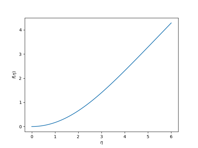
In fluid mechanics the Blasius equation comes up (http://en.wikipedia.org/wiki/Blasius_boundary_layer) to describe the boundary layer that forms near a flat plate with fluid moving by it. The nonlinear differential equation is:

\begin{eqnarray} f''' + \frac{1}{2} f f'' &=& 0 \\ f(0) &=& 0 \\ f'(0) &=& 0 \\ f'(\infty) &=& 1 \end{eqnarray}

This is a nonlinear, boundary value problem. The point of solving this equation is to get the value of \(f''(0)\) to evaluate the shear stress at the plate.

We have to convert this to a system of first-order differential equations. Let \(f_1 = f\), \(f_2 = f_1'\) and \(f_3 = f_2'\). This leads to:

\begin{eqnarray} f_1' = f_2 \\ f_2' = f_3 \\ f_3' = -\frac{1}{2} f_1 f_3 \\ f_1(0) = 0 \\ f_2(0) = 0 \\ f_2(\infty) = 1 \end{eqnarray}

It is not possible to specify a boundary condition at \(\infty\) numerically, so we will have to use a large number, and verify it is "large enough". From the solution, we evaluate the derivatives at \(\eta=0\), and we have \(f''(0) = f_3(0)\).

We have to provide initial guesses for f_1, f_2 and f_3. This is the hardest part about this problem. We know that f_1 starts at zero, and is flat there (f'(0)=0), but at large eta, it has a constant slope of one. We will guess a simple line of slope = 1 for f_1. That is correct at large eta, and is zero at η=0. If the slope of the function is constant at large \(\eta\), then the values of higher derivatives must tend to zero. We choose an exponential decay as a guess.

Finally, we let a solver iteratively find a solution for us, and find the answer we want. The solver is in the pycse module.

import numpy as np
from pycse import bvp

def odefun(F, x):
    f1, f2, f3 = F.T
    return np.column_stack([f2,
                            f3,
                            -0.5 * f1 * f3])

def bcfun(Y):
    fa, fb = Y[0, :], Y[-1, :]
    return [fa[0],        # f1(0) =  0
            fa[1],        # f2(0) = 0
            1.0 - fb[1]]  # f2(inf) = 1

eta = np.linspace(0, 6, 100)
f1init = eta
f2init = np.exp(-eta)
f3init = np.exp(-eta)

Finit = np.column_stack([f1init, f2init, f3init])

sol = bvp(odefun, bcfun, eta, Finit)
f1, f2, f3 = sol.T

print("f''(0) = f_3(0) = {0}".format(f3[0]))

import matplotlib.pyplot as plt
plt.plot(eta, f1)
plt.xlabel('$\eta$')
plt.ylabel('$f(\eta)$')
plt.savefig('images/blasius.png')
f''(0) = f_3(0) = 0.3324911095517483

<2017-05-17 Wed> You need pycse 1.6.4 for this example.

Copyright (C) 2017 by John Kitchin. See the License for information about copying.

org-mode source

Org-mode version = 9.1.2

Discuss on Twitter

Another look at nonlinear BVPs

| categories: bvp | tags:

Adapted from http://www.mathworks.com/help/matlab/ref/bvp4c.html

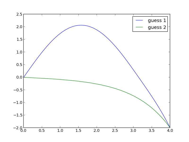
Boundary value problems may have more than one solution. Let us consider the BVP:

\begin{eqnarray} y'' + |y| &=& 0 \\ y(0) &=& 0 \\ y(4) &=& -2 \end{eqnarray}

We will see this equation has two answers, depending on your initial guess. We convert this to the following set of coupled equations:

\begin{eqnarray} y_1' &=& y_2 \\ y_2' &=& -|y_1| \\ y_1(0)&=& 0\\ y_1(4) &=& -2 \end{eqnarray}

This BVP is nonlinear because of the absolute value. We will have to guess solutions to get started. We will guess two different solutions, both of which will be constant values. We will use pycse.bvp to solve the equation.

import numpy as np
from pycse import bvp
import matplotlib.pyplot as plt

def odefun(Y, x):
    y1, y2 = Y
    dy1dx = y2
    dy2dx = -np.abs(y1)
    return [dy1dx, dy2dx]

def bcfun(Ya, Yb):
    y1a, y2a = Ya
    y1b, y2b = Yb

    return [y1a, -2 - y1b]

x = np.linspace(0, 4, 100)

y1 = 1.0 * np.ones(x.shape)
y2 = 0.0 * np.ones(x.shape)

Yinit = np.vstack([y1, y2])

sol = bvp(odefun, bcfun, x, Yinit)

plt.plot(x, sol[0])

# another initial guess
y1 = -1.0 * np.ones(x.shape)
y2 = 0.0 * np.ones(x.shape)

Yinit = np.vstack([y1, y2])

sol = bvp(odefun, bcfun, x, Yinit)

plt.plot(x, sol[0])
plt.legend(['guess 1', 'guess 2'])
plt.savefig('images/bvp-another-nonlin-1.png')
plt.show()

This example shows that a nonlinear BVP may have different solutions, and which one you get depends on the guess you make for the solution. This is analogous to solving nonlinear algebraic equations (which is what is done in solving this problem!).

Copyright (C) 2013 by John Kitchin. See the License for information about copying.

org-mode source

Discuss on Twitter

Numerical Simpsons rule

| categories: math, integration | tags:

A more accurate numerical integration than the trapezoid method is Simpson's rule. The syntax is similar to trapz, but the method is in scipy.integrate.

import numpy as np
from scipy.integrate import simps, romb

a = 0.0; b = np.pi / 4.0;
N = 10  # this is the number of intervals

x = np.linspace(a, b, N)
y = np.cos(x)

t = np.trapz(y, x)
s = simps(y, x)
a = np.sin(b) - np.sin(a)

print
print 'trapz = {0} ({1:%} error)'.format(t, (t - a)/a)
print 'simps = {0} ({1:%} error)'.format(s, (s - a)/a)
print 'analy = {0}'.format(a)
>>> >>> >>> >>> >>> >>> >>> >>> >>> >>> >>> >>>
trapz = 0.70665798038 (-0.063470% error)
simps = 0.707058914216 (-0.006769% error)
analy = 0.707106781187

You can see the Simpson's method is more accurate than the trapezoid method.

Copyright (C) 2013 by John Kitchin. See the License for information about copying.

org-mode source

Discuss on Twitter
« Previous Page -- Next Page »