Solving integral equations with fsolve

| categories: nonlinear algebra | tags: reaction engineering

Original post in Matlab

Occasionally we have integral equations we need to solve in engineering problems, for example, the volume of plug flow reactor can be defined by this equation: \(V = \int_{Fa(V=0)}^{Fa} \frac{1}{r_a} dFa\) where \(r_a\) is the rate law. Suppose we know the reactor volume is 100 L, the inlet molar flow of A is 1 mol/L, the volumetric flow is 10 L/min, and \(r_a = -k Ca\), with \(k=0.23\) 1/min. What is the exit molar flow rate? We need to solve the following equation:

$$100 = \int_{Fa(V=0)}^{Fa} \frac{1}{-k Fa/\nu} dFa$$

We start by creating a function handle that describes the integrand. We can use this function in the quad command to evaluate the integral.

import numpy as np
from scipy.integrate import quad
from scipy.optimize import fsolve

k = 0.23
nu = 10.0
Fao = 1.0

def integrand(Fa):
    return -1.0 / (k * Fa / nu)

def func(Fa):
    integral,err = quad(integrand, Fao, Fa)
    return 100.0 - integral

vfunc = np.vectorize(func)

We will need an initial guess, so we make a plot of our function to get an idea.

import matplotlib.pyplot as plt

f = np.linspace(0.01, 1)
plt.plot(f, vfunc(f))
plt.xlabel('Molar flow rate')
plt.savefig('images/integral-eqn-guess.png')
plt.show()
>>> >>> [<matplotlib.lines.Line2D object at 0x964a910>]
<matplotlib.text.Text object at 0x961fe50>

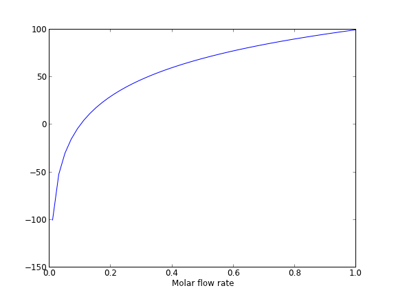
Now we can see a zero is near Fa = 0.1, so we proceed to solve the equation.

Fa_guess = 0.1
Fa_exit, = fsolve(vfunc, Fa_guess)
print 'The exit concentration is {0:1.2f} mol/L'.format(Fa_exit / nu)
>>> The exit concentration is 0.01 mol/L

1 Summary notes

This example seemed a little easier in Matlab, where the quad function seemed to get automatically vectorized. Here we had to do it by hand.

Copyright (C) 2013 by John Kitchin. See the License for information about copying.

org-mode source

Discuss on Twitter

Polynomials in python

| categories: math, polynomials | tags:

Matlab post

Polynomials can be represented as a list of coefficients. For example, the polynomial \(4*x^3 + 3*x^2 -2*x + 10 = 0\) can be represented as [4, 3, -2, 10]. Here are some ways to create a polynomial object, and evaluate it.

import numpy as np

ppar = [4, 3, -2, 10]
p = np.poly1d(ppar)

print p(3)
print np.polyval(ppar, 3)

x = 3
print 4*x**3 + 3*x**2 -2*x + 10
139
139
139

numpy makes it easy to get the derivative and integral of a polynomial.

Consider: \(y = 2x^2 - 1\). We know the derivative is \(4x\). Here we compute the derivative and evaluate it at x=4.

import numpy as np

p = np.poly1d([2, 0, -1])
p2 = np.polyder(p)
print p2
print p2(4)
 
4 x
16

The integral of the previous polynomial is \(\frac{2}{3} x^3 - x + c\). We assume \(C=0\). Let us compute the integral \(\int_2^4 2x^2 - 1 dx\).

import numpy as np

p = np.poly1d([2, 0, -1])
p2 = np.polyint(p)
print p2
print p2(4) - p2(2)
        3
0.6667 x - 1 x
35.3333333333

One reason to use polynomials is the ease of finding all of the roots using numpy.roots.

import numpy as np
print np.roots([2, 0, -1]) # roots are +- sqrt(2)

# note that imaginary roots exist, e.g. x^2 + 1 = 0 has two roots, +-i
p = np.poly1d([1, 0, 1])
print np.roots(p)
[ 0.70710678 -0.70710678]
[ 0.+1.j  0.-1.j]

There are applications of polynomials in thermodynamics. The van der waal equation is a cubic polynomial \(f(V) = V^3 - \frac{p n b + n R T}{p} V^2 + \frac{n^2 a}{p}V - \frac{n^3 a b}{p} = 0\), where \(a\) and \(b\) are constants, \(p\) is the pressure, \(R\) is the gas constant, \(T\) is an absolute temperature and \(n\) is the number of moles. The roots of this equation tell you the volume of the gas at those conditions.

import numpy as np
# numerical values of the constants
a = 3.49e4
b = 1.45
p = 679.7   # pressure in psi
T = 683     # T in Rankine
n = 1.136   # lb-moles
R = 10.73       # ft^3 * psi /R / lb-mol

ppar = [1.0, -(p*n*b+n*R*T)/p, n**2*a/p,  -n**3*a*b/p];
print np.roots(ppar)
[ 5.09432376+0.j          4.40066810+1.43502848j  4.40066810-1.43502848j]

Note that only one root is real (and even then, we have to interpet 0.j as not being imaginary. Also, in a cubic polynomial, there can only be two imaginary roots). In this case that means there is only one phase present.

1 Summary

Polynomials in numpy are even better than in Matlab, because you get a polynomial object that acts just like a function. Otherwise, they are functionally equivalent.

Copyright (C) 2013 by John Kitchin. See the License for information about copying.

org-mode source

Discuss on Twitter

Controlling the format of printed variables

| categories: python | tags:

This was first worked out in this original Matlab post.

Often you will want to control the way a variable is printed. You may want to only show a few decimal places, or print in scientific notation, or embed the result in a string. Here are some examples of printing with no control over the format.

a = 2./3
print a
print 1/3
print 1./3.
print 10.1
print "Avogadro's number is ", 6.022e23,'.'
0.666666666667
0
0.333333333333
10.1
Avogadro's number is  6.022e+23 .

There is no control over the number of decimals, or spaces around a printed number.

In python, we use the format function to control how variables are printed. With the format function you use codes like {n:format specifier} to indicate that a formatted string should be used. n is the n^{th} argument passed to format, and there are a variety of format specifiers. Here we examine how to format float numbers. The specifier has the general form “w.df” where w is the width of the field, and d is the number of decimals, and f indicates a float number. “1.3f” means to print a float number with 3 decimal places. Here is an example.

print 'The value of 1/3 to 3 decimal places is {0:1.3f}'.format(1./3.)
The value of 1/3 to 3 decimal places is 0.333

In that example, the 0 in {0:1.3f} refers to the first (and only) argument to the format function. If there is more than one argument, we can refer to them like this:

print 'Value 0 = {0:1.3f}, value 1 = {1:1.3f}, value 0 = {0:1.3f}'.format(1./3., 1./6.)
Value 0 = 0.333, value 1 = 0.167, value 0 = 0.333

Note you can refer to the same argument more than once, and in arbitrary order within the string.

Suppose you have a list of numbers you want to print out, like this:

for x in [1./3., 1./6., 1./9.]:
    print 'The answer is {0:1.2f}'.format(x)
The answer is 0.33
The answer is 0.17
The answer is 0.11

The “g” format specifier is a general format that can be used to indicate a precision, or to indicate significant digits. To print a number with a specific number of significant digits we do this:

print '{0:1.3g}'.format(1./3.)
print '{0:1.3g}'.format(4./3.)
0.333
1.33

We can also specify plus or minus signs. Compare the next two outputs.

for x in [-1., 1.]: 
    print '{0:1.2f}'.format(x)
-1.00
1.00

You can see the decimals do not align. That is because there is a minus sign in front of one number. We can specify to show the sign for positive and negative numbers, or to pad positive numbers to leave space for positive numbers.

for x in [-1., 1.]: 
    print '{0:+1.2f}'.format(x) # explicit sign

for x in [-1., 1.]: 
    print '{0: 1.2f}'.format(x) # pad positive numbers
-1.00
+1.00
-1.00
 1.00

We use the “e” or “E” format modifier to specify scientific notation.

import numpy as np
eps = np.finfo(np.double).eps
print eps
print '{0}'.format(eps)
print '{0:1.2f}'.format(eps)
print '{0:1.2e}'.format(eps)  #exponential notation
print '{0:1.2E}'.format(eps)  #exponential notation with capital E
2.22044604925e-16
2.22044604925e-16
0.00
2.22e-16
2.2E-16

As a float with 2 decimal places, that very small number is practically equal to 0.

We can even format percentages. Note you do not need to put the % in your string.

print 'the fraction {0} corresponds to {0:1.0%}'.format(0.78)
the fraction 0.78 corresponds to 78%

There are many other options for formatting strings. See http://docs.python.org/2/library/string.html#formatstrings for a full specification of the options.

Copyright (C) 2013 by John Kitchin. See the License for information about copying.

org-mode source

Discuss on Twitter

Integrating equations in python

| categories: integration, python | tags:

A common need in engineering calculations is to integrate an equation over some range to determine the total change. For example, say we know the volumetric flow changes with time according to \(d\nu/dt = \alpha t\), where \(\alpha = 1\) L/min and we want to know how much liquid flows into a tank over 10 minutes if the volumetric flowrate is \(\nu_0 = 5\) L/min at \(t=0\). The answer to that question is the value of this integral: \(V = \int_0^{10} \nu_0 + \alpha t dt\).

import scipy
from scipy.integrate import quad

nu0 = 5     # L/min
alpha = 1.0 # L/min
def integrand(t):
    return nu0 + alpha * t

t0 = 0.0
tfinal = 10.0
V, estimated_error = quad(integrand, t0, tfinal)
print('{0:1.2f} L flowed into the tank over 10 minutes'.format(V))
100.00 L flowed into the tank over 10 minutes

That is all there is too it!

Copyright (C) 2013 by John Kitchin. See the License for information about copying.

org-mode source

Discuss on Twitter

Using units in python

| categories: units, python | tags:

Units in Matlab

I think an essential feature in an engineering computational environment is properly handling units and unit conversions. Mathcad supports that pretty well. I wrote a package for doing it in Matlab. Today I am going to explore units in python. Here are some of the packages that I have found which support units to some extent

  1. http://pypi.python.org/pypi/units/
  2. http://packages.python.org/quantities/user/tutorial.html
  3. http://dirac.cnrs-orleans.fr/ScientificPython/ScientificPythonManual/Scientific.Physics.PhysicalQuantities-module.html
  4. http://home.scarlet.be/be052320/Unum.html
  5. https://simtk.org/home/python_units
  6. http://docs.enthought.com/scimath/units/intro.html

The last one looks most promising.

import numpy as np
from scimath.units.volume import liter
from scimath.units.substance import mol

q = np.array([1, 2, 3]) * mol
print q

P = q / liter
print P
[1.0*mol 2.0*mol 3.0*mol]
[1000.0*m**-3*mol 2000.0*m**-3*mol 3000.0*m**-3*mol]

That doesn't look too bad. It is a little clunky to have to import every unit, and it is clear the package is saving everything in SI units by default. Let us try to solve an equation.

Find the time that solves this equation.

\(0.01 = C_{A0} e^{-kt}\)

First we solve without units. That way we know the answer.

import numpy as np
from scipy.optimize import fsolve

CA0 = 1.0  # mol/L
CA = 0.01  # mol/L
k = 1.0    # 1/s

def func(t):
    z = CA - CA0 * np.exp(-k*t)
    return z

t0 = 2.3

t, = fsolve(func, t0)
print 't = {0:1.2f} seconds'.format(t)
t = 4.61 seconds

Now, with units. I note here that I tried the obvious thing of just importing the units, and adding them on, but the package is unable to work with floats that have units. For some functions, there must be an ndarray with units which is practically what the UnitScalar code below does.

import numpy as np
from scipy.optimize import fsolve
from scimath.units.volume import liter
from scimath.units.substance import mol
from scimath.units.time import second
from scimath.units.api import has_units, UnitScalar

CA0 = UnitScalar(1.0, units = mol / liter)
CA = UnitScalar(0.01, units = mol / liter)
k = UnitScalar(1.0, units = 1 / second)

@has_units(inputs="t::units=s",
           outputs="result::units=mol/liter")
def func(t):
    z = CA - CA0 * float(np.exp(-k*t))
    return z

t0 = UnitScalar(2.3, units = second)

t, = fsolve(func, t0)
print 't = {0:1.2f} seconds'.format(t)
print type(t)
t = 4.61 seconds
<type 'numpy.float64'>

This is some heavy syntax that in the end does not preserve the units. In my Matlab package, we had to “wrap” many functions like fsolve so they would preserve units. Clearly this package will need that as well. Overall, in its current implementation this package does not do what I would expect all the time.1

Copyright (C) 2013 by John Kitchin. See the License for information about copying.

org-mode source

Discuss on Twitter
« Previous Page -- Next Page »