Vectorized piecewise functions

| categories: math | tags:

Matlab post Occasionally we need to define piecewise functions, e.g.

\begin{eqnarray} f(x) &=& 0, x < 0 \\ &=& x, 0 <= x < 1\\ &=& 2 - x, 1 < x <= 2\\ &=& 0, x > 2 \end{eqnarray}

Today we examine a few ways to define a function like this. A simple way is to use conditional statements.

def f1(x):
    if x < 0:
        return 0
    elif (x >= 0) & (x < 1):
        return x
    elif (x >= 1) & (x < 2):
        return 2.0 - x
    else:
        return 0

print f1(-1)
print f1([0, 1, 2, 3])  # does not work!
... ... ... ... ... ... ... ... >>> 0
0

This works, but the function is not vectorized, i.e. f([-1 0 2 3]) does not evaluate properly (it should give a list or array). You can get vectorized behavior by using list comprehension, or by writing your own loop. This does not fix all limitations, for example you cannot use the f1 function in the quad function to integrate it.

import numpy as np
import matplotlib.pyplot as plt

x = np.linspace(-1, 3)
y = [f1(xx) for xx in x]

plt.plot(x, y)
plt.savefig('images/vector-piecewise.png')
>>> >>> >>> >>> >>> [<matplotlib.lines.Line2D object at 0x048D6790>]

Neither of those methods is convenient. It would be nicer if the function was vectorized, which would allow the direct notation f1([0, 1, 2, 3, 4]). A simple way to achieve this is through the use of logical arrays. We create logical arrays from comparison statements.

def f2(x):
    'fully vectorized version'
    x = np.asarray(x)
    y = np.zeros(x.shape)
    y += ((x >= 0) & (x < 1)) * x
    y += ((x >= 1) & (x < 2)) * (2 - x)
    return y

print f2([-1, 0, 1, 2, 3, 4])
x = np.linspace(-1,3);
plt.plot(x,f2(x))
plt.savefig('images/vector-piecewise-2.png')
... ... ... ... ... ... >>> [ 0.  0.  1.  0.  0.  0.]
>>> [<matplotlib.lines.Line2D object at 0x043A4910>]

A third approach is to use Heaviside functions. The Heaviside function is defined to be zero for x less than some value, and 0.5 for x=0, and 1 for x >= 0. If you can live with y=0.5 for x=0, you can define a vectorized function in terms of Heaviside functions like this.

def heaviside(x):
    x = np.array(x)
    if x.shape != ():
        y = np.zeros(x.shape)
        y[x > 0.0] = 1
        y[x == 0.0] = 0.5
    else: # special case for 0d array (a number)
        if x > 0: y = 1
        elif x == 0: y = 0.5
        else: y = 0
    return y

def f3(x):
    x = np.array(x)
    y1 = (heaviside(x) - heaviside(x - 1)) * x # first interval
    y2 = (heaviside(x - 1) - heaviside(x - 2)) * (2 - x) # second interval
    return y1 + y2

from scipy.integrate import quad
print quad(f3, -1, 3)
... ... ... ... ... ... ... ... ... ... >>> ... ... ... ... ... >>> >>> (1.0, 1.1102230246251565e-14)
plt.plot(x, f3(x))
plt.savefig('images/vector-piecewise-3.png')
[<matplotlib.lines.Line2D object at 0x048F96F0>]

There are many ways to define piecewise functions, and vectorization is not always necessary. The advantages of vectorization are usually notational simplicity and speed; loops in python are usually very slow compared to vectorized functions.

Copyright (C) 2013 by John Kitchin. See the License for information about copying.

org-mode source

Discuss on Twitter

The trapezoidal method of integration

| categories: math, integration | tags:

Matlab post See http://en.wikipedia.org/wiki/Trapezoidal_rule

$$\int_a^b f(x) dx \approx \frac{1}{2}\displaystyle\sum\limits_{k=1}^N(x_{k+1}-x_k)(f(x_{k+1}) + f(x_k))$$

Let us compute the integral of sin(x) from x=0 to \(\pi\). To approximate the integral, we need to divide the interval from \(a\) to \(b\) into \(N\) intervals. The analytical answer is 2.0.

We will use this example to illustrate the difference in performance between loops and vectorized operations in python.

import numpy as np
import time

a = 0.0; b = np.pi;
N = 1000; # this is the number of intervals

h = (b - a)/N; # this is the width of each interval
x = np.linspace(a, b, N) 
y = np.sin(x); # the sin function is already vectorized

t0 = time.time()
f = 0.0
for k in range(len(x) - 1):
    f += 0.5 * ((x[k+1] - x[k]) * (y[k+1] + y[k]))

tf = time.time() - t0
print 'time elapsed = {0} sec'.format(tf)

print f
>>> >>> >>> >>> >>> >>> >>> >>> >>> >>> >>> ... ... >>> >>> time elapsed = 0.0780000686646 sec
>>> 1.99999835177
t0 = time.time()
Xk = x[1:-1] - x[0:-2] # vectorized version of (x[k+1] - x[k])
Yk = y[1:-1] + y[0:-2] # vectorized version of (y[k+1] + y[k])

f = 0.5 * np.sum(Xk * Yk) # vectorized version of the loop above
tf = time.time() - t0
print 'time elapsed = {0} sec'.format(tf)

print f
>>> >>> >>> >>> >>> time elapsed = 0.077999830246 sec
>>> 1.99999340709

In the last example, there may be loop buried in the sum command. Let us do one final method, using linear algebra, in a single line. The key to understanding this is to recognize the sum is just the result of a dot product of the x differences and y sums.

t0 = time.time()
f = 0.5 * np.dot(Xk, Yk)
tf = time.time() - t0
print 'time elapsed = {0} sec'.format(tf)

print f
>>> >>> time elapsed = 0.0310001373291 sec
>>> 1.99999340709

The loop method is straightforward to code, and looks alot like the formula that defines the trapezoid method. the vectorized methods are not as easy to read, and take fewer lines of code to write. However, the vectorized methods are much faster than the loop, so the loss of readability could be worth it for very large problems.

The times here are considerably slower than in Matlab. I am not sure if that is a totally fair comparison. Here I am running python through emacs, which may result in slower performance. I also used a very crude way of timing the performance which lumps some system performance in too.

Copyright (C) 2013 by John Kitchin. See the License for information about copying.

org-mode source

Discuss on Twitter

Method of continuity for nonlinear equation solving

| categories: nonlinear algebra | tags:

Matlab post Adapted from Perry's Chemical Engineers Handbook, 6th edition 2-63.

We seek the solution to the following nonlinear equations:

\(2 + x + y - x^2 + 8 x y + y^3 = 0\)

\(1 + 2x - 3y + x^2 + xy - y e^x = 0\)

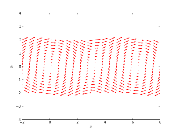
In principle this is easy, we simply need some initial guesses and a nonlinear solver. The challenge here is what would you guess? There could be many solutions. The equations are implicit, so it is not easy to graph them, but let us give it a shot, starting on the x range -5 to 5. The idea is set a value for x, and then solve for y in each equation.

import numpy as np
from scipy.optimize import fsolve

import matplotlib.pyplot as plt

def f(x, y):
    return 2 + x + y - x**2 + 8*x*y + y**3;

def g(x, y):
    return 1 + 2*x - 3*y + x**2 + x*y - y*np.exp(x)

x = np.linspace(-5, 5, 500)

@np.vectorize
def fy(x):
    x0 = 0.0
    def tmp(y):
        return f(x, y)
    y1, = fsolve(tmp, x0)
    return y1

@np.vectorize
def gy(x):
    x0 = 0.0
    def tmp(y):
        return g(x, y)
    y1, = fsolve(tmp, x0)
    return y1


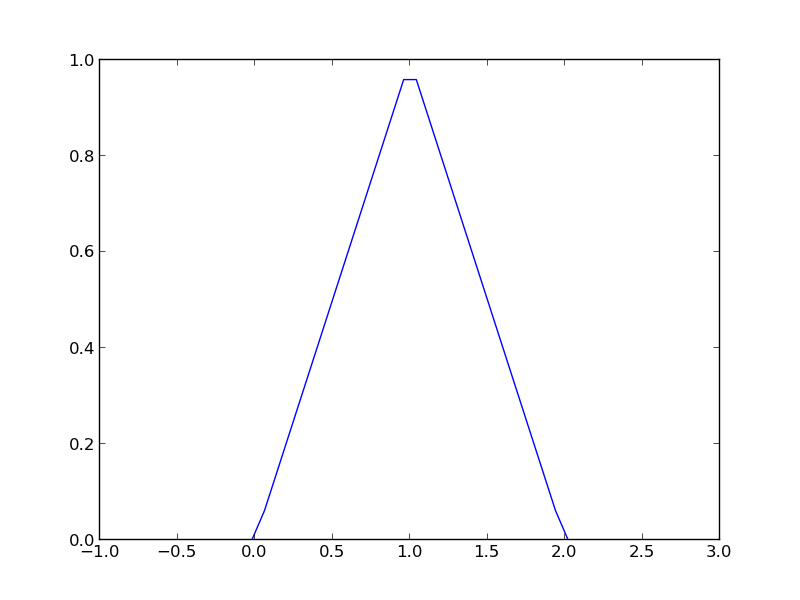
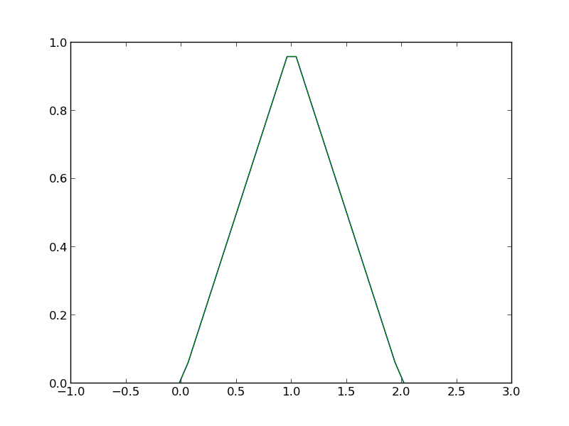
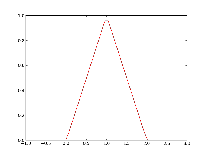
plt.plot(x, fy(x), x, gy(x))
plt.xlabel('x')
plt.ylabel('y')
plt.legend(['fy', 'gy'])
plt.savefig('images/continuation-1.png')
>>> >>> >>> >>> ... ... >>> ... ... >>> >>> >>> ... ... ... ... ... ... ... >>> ... ... ... ... ... ... ... >>> >>> /opt/kitchingroup/enthought/epd-7.3-2-rh5-x86_64/lib/python2.7/site-packages/scipy/optimize/minpack.py:152: RuntimeWarning: The iteration is not making good progress, as measured by the 
  improvement from the last ten iterations.
  warnings.warn(msg, RuntimeWarning)
/opt/kitchingroup/enthought/epd-7.3-2-rh5-x86_64/lib/python2.7/site-packages/scipy/optimize/minpack.py:152: RuntimeWarning: The iteration is not making good progress, as measured by the 
  improvement from the last five Jacobian evaluations.
  warnings.warn(msg, RuntimeWarning)
[<matplotlib.lines.Line2D object at 0x1a0c4990>, <matplotlib.lines.Line2D object at 0x1a0c4a90>]
<matplotlib.text.Text object at 0x19d5e390>
<matplotlib.text.Text object at 0x19d61d90>
<matplotlib.legend.Legend object at 0x189df850>

You can see there is a solution near x = -1, y = 0, because both functions equal zero there. We can even use that guess with fsolve. It is disappointly easy! But, keep in mind that in 3 or more dimensions, you cannot perform this visualization, and another method could be required.

def func(X):
    x,y = X
    return [f(x, y), g(x, y)]

print fsolve(func, [-2, -2])
... ... >>> [ -1.00000000e+00   1.28730858e-15]

We explore a method that bypasses this problem today. The principle is to introduce a new variable, \(\lambda\), which will vary from 0 to 1. at \(\lambda=0\) we will have a simpler equation, preferrably a linear one, which can be easily solved, or which can be analytically solved. At \(\lambda=1\), we have the original equations. Then, we create a system of differential equations that start at the easy solution, and integrate from \(\lambda=0\) to \(\lambda=1\), to recover the final solution.

We rewrite the equations as:

\(f(x,y) = (2 + x + y) + \lambda(- x^2 + 8 x y + y^3) = 0\)

\(g(x,y) = (1 + 2x - 3y) + \lambda(x^2 + xy - y e^x) = 0\)

Now, at \(\lambda=0\) we have the simple linear equations:

\(x + y = -2\)

\(2x - 3y = -1\)

These equations are trivial to solve:

x0 = np.linalg.solve([[1., 1.], [2., -3.]],[ -2, -1])
print x0
[-1.4 -0.6]

We form the system of ODEs by differentiating the new equations with respect to \(\lambda\). Why do we do that? The solution, (x,y) will be a function of \(\lambda\). From calculus, you can show that:

\(\frac{\partial f}{\partial x}\frac{\partial x}{\partial \lambda}+\frac{\partial f}{\partial y}\frac{\partial y}{\partial \lambda}=-\frac{\partial f}{\partial \lambda}\)

\(\frac{\partial g}{\partial x}\frac{\partial x}{\partial \lambda}+\frac{\partial g}{\partial y}\frac{\partial y}{\partial \lambda}=-\frac{\partial g}{\partial \lambda}\)

Now, solve this for \(\frac{\partial x}{\partial \lambda}\) and \(\frac{\partial y}{\partial \lambda}\). You can use Cramer's rule to solve for these to yield:

\begin{eqnarray} \ \frac{\partial x}{\partial \lambda} &=& \frac{\partial f/\partial y \partial g/\partial \lambda - \partial f/\partial \lambda \partial g/\partial y}{\partial f/\partial x \partial g/\partial y - \partial f/\partial y \partial g/\partial x } \\\\ \frac{\partial y}{\partial \lambda} &=& \frac{\partial f/\partial \lambda \partial g/\partial x - \partial f/\partial x \partial g/\partial \lambda}{\partial f/\partial x \partial g/\partial y - \partial f/\partial y \partial g/\partial x } \end{eqnarray} For this set of equations: \begin{eqnarray} \ \partial f/\partial x &=& 1 - 2\lambda x + 8\lambda y \\\\ \partial f/\partial y &=& 1 + 8 \lambda x + 3 \lambda y^2 \\\\ \partial g/\partial x &=& 2 + 2 \lambda x + \lambda y - \lambda y e^x\\\\ \partial g/\partial y &=& -3 + \lambda x - \lambda e^x \end{eqnarray}

Now, we simply set up those two differential equations on \(\frac{\partial x}{\partial \lambda}\) and \(\frac{\partial y}{\partial \lambda}\), with the initial conditions at \(\lambda = 0\) which is the solution of the simpler linear equations, and integrate to \(\lambda = 1\), which is the final solution of the original equations!

def ode(X, LAMBDA):
    x,y = X
    pfpx = 1.0 - 2.0 * LAMBDA * x + 8 * LAMBDA * y
    pfpy = 1.0 + 8.0 * LAMBDA * x + 3.0 * LAMBDA * y**2
    pfpLAMBDA = -x**2 + 8.0 * x * y + y**3;
    pgpx = 2. + 2. * LAMBDA * x + LAMBDA * y - LAMBDA * y * np.exp(x)
    pgpy = -3. + LAMBDA * x - LAMBDA * np.exp(x)
    pgpLAMBDA = x**2 + x * y - y * np.exp(x);
    dxdLAMBDA = (pfpy * pgpLAMBDA - pfpLAMBDA * pgpy) / (pfpx * pgpy - pfpy * pgpx)
    dydLAMBDA = (pfpLAMBDA * pgpx - pfpx * pgpLAMBDA) / (pfpx * pgpy - pfpy * pgpx) 
    dXdLAMBDA = [dxdLAMBDA, dydLAMBDA]
    return dXdLAMBDA


from scipy.integrate import odeint

lambda_span = np.linspace(0, 1, 100)

X = odeint(ode, x0, lambda_span)

xsol, ysol = X[-1]
print 'The solution is at x={0:1.3f}, y={1:1.3f}'.format(xsol, ysol)
print f(xsol, ysol), g(xsol, ysol)
... ... ... ... ... ... ... ... ... >>> >>> >>> >>> >>> >>> >>> The solution is at x=-1.000, y=0.000
-1.27746598808e-06 -1.15873819107e-06

You can see the solution is somewhat approximate; the true solution is x = -1, y = 0. The approximation could be improved by lowering the tolerance on the ODE solver. The functions evaluate to a small number, close to zero. You have to apply some judgment to determine if that is sufficiently accurate. For instance if the units on that answer are kilometers, but you need an answer accurate to a millimeter, this may not be accurate enough.

This is a fair amount of work to get a solution! The idea is to solve a simple problem, and then gradually turn on the hard part by the lambda parameter. What happens if there are multiple solutions? The answer you finally get will depend on your \(\lambda=0\) starting point, so it is possible to miss solutions this way. For problems with lots of variables, this would be a good approach if you can identify the easy problem.

Copyright (C) 2013 by John Kitchin. See the License for information about copying.

org-mode source

Discuss on Twitter

ODEs with discontinuous forcing functions

| categories: ode | tags:

Matlab post

Adapted from http://archives.math.utk.edu/ICTCM/VOL18/S046/paper.pdf

A mixing tank initially contains 300 g of salt mixed into 1000 L of water. At t=0 min, a solution of 4 g/L salt enters the tank at 6 L/min. At t=10 min, the solution is changed to 2 g/L salt, still entering at 6 L/min. The tank is well stirred, and the tank solution leaves at a rate of 6 L/min. Plot the concentration of salt (g/L) in the tank as a function of time.

A mass balance on the salt in the tank leads to this differential equation: \(\frac{dM_S}{dt} = \nu C_{S,in}(t) - \nu M_S/V\) with the initial condition that \(M_S(t=0)=300\). The wrinkle is that the inlet conditions are not constant.

$$C_{S,in}(t) = \begin{array}{ll} 0 & t \le 0, \\ 4 & 0 < t \le 10, \\ 2 & t > 10. \end{array}$$

import numpy as np
from scipy.integrate import odeint
import matplotlib.pyplot as plt

V = 1000.0 # L
nu = 6.0  # L/min
    
def Cs_in(t):
    'inlet concentration'
    if t < 0:
        Cs = 0.0 # g/L
    elif (t > 0) and (t <= 10):
        Cs = 4.0
    else:
        Cs = 2.0
    return Cs

def mass_balance(Ms, t):
    '$\frac{dM_S}{dt} = \nu C_{S,in}(t) - \nu M_S/V$'
    dMsdt = nu * Cs_in(t) - nu * Ms / V
    return dMsdt

tspan = np.linspace(0.0, 15.0, 50)

M0 = 300.0 # gm salt
Ms = odeint(mass_balance, M0, tspan)

plt.plot(tspan, Ms/V, 'b.-')
plt.xlabel('Time (min)')
plt.ylabel('Salt concentration (g/L)')
plt.savefig('images/ode-discont.png')

You can see the discontinuity in the salt concentration at 10 minutes due to the discontinous change in the entering salt concentration.

Copyright (C) 2013 by John Kitchin. See the License for information about copying.

org-mode source

Discuss on Twitter

Phase portraits of a system of ODEs

| categories: math, ode | tags:

Matlab post An undamped pendulum with no driving force is described by

$$ y'' + sin(y) = 0$$

We reduce this to standard matlab form of a system of first order ODEs by letting \(y_1 = y\) and \(y_2=y_1'\). This leads to:

\(y_1' = y_2\)

\(y_2' = -sin(y_1)\)

The phase portrait is a plot of a vector field which qualitatively shows how the solutions to these equations will go from a given starting point. here is our definition of the differential equations:

To generate the phase portrait, we need to compute the derivatives \(y_1'\) and \(y_2'\) at \(t=0\) on a grid over the range of values for \(y_1\) and \(y_2\) we are interested in. We will plot the derivatives as a vector at each (y1, y2) which will show us the initial direction from each point. We will examine the solutions over the range -2 < y1 < 8, and -2 < y2 < 2 for y2, and create a grid of 20 x 20 points.

import numpy as np
import matplotlib.pyplot as plt

def f(Y, t):
    y1, y2 = Y
    return [y2, -np.sin(y1)]

y1 = np.linspace(-2.0, 8.0, 20)
y2 = np.linspace(-2.0, 2.0, 20)

Y1, Y2 = np.meshgrid(y1, y2)

t = 0

u, v = np.zeros(Y1.shape), np.zeros(Y2.shape)

NI, NJ = Y1.shape

for i in range(NI):
    for j in range(NJ):
        x = Y1[i, j]
        y = Y2[i, j]
        yprime = f([x, y], t)
        u[i,j] = yprime[0]
        v[i,j] = yprime[1]
     

Q = plt.quiver(Y1, Y2, u, v, color='r')

plt.xlabel('$y_1$')
plt.ylabel('$y_2$')
plt.xlim([-2, 8])
plt.ylim([-4, 4])
plt.savefig('images/phase-portrait.png')
>>> ... >>> >>> >>> >>> >>> >>> ... ... ... >>> >>> <matplotlib.text.Text object at 0xbcfd290>
<matplotlib.text.Text object at 0xbd14750>
(-2, 8)
(-4, 4)

Let us plot a few solutions on the vector field. We will consider the solutions where y1(0)=0, and values of y2(0) = [0 0.5 1 1.5 2 2.5], in otherwords we start the pendulum at an angle of zero, with some angular velocity.

from scipy.integrate import odeint

for y20 in [0, 0.5, 1, 1.5, 2, 2.5]:
    tspan = np.linspace(0, 50, 200)
    y0 = [0.0, y20]
    ys = odeint(f, y0, tspan)
    plt.plot(ys[:,0], ys[:,1], 'b-') # path
    plt.plot([ys[0,0]], [ys[0,1]], 'o') # start
    plt.plot([ys[-1,0]], [ys[-1,1]], 's') # end
    

plt.xlim([-2, 8])
plt.savefig('images/phase-portrait-2.png')
plt.show()
>>> ... ... ... [<matplotlib.lines.Line2D object at 0xbc0dbd0>]
[<matplotlib.lines.Line2D object at 0xc135050>]
[<matplotlib.lines.Line2D object at 0xbd1a450>]
[<matplotlib.lines.Line2D object at 0xbd1a1d0>]
[<matplotlib.lines.Line2D object at 0xb88aa10>]
[<matplotlib.lines.Line2D object at 0xb88a5d0>]
[<matplotlib.lines.Line2D object at 0xc14e410>]
[<matplotlib.lines.Line2D object at 0xc14ed90>]
[<matplotlib.lines.Line2D object at 0xc2c5290>]
[<matplotlib.lines.Line2D object at 0xbea4bd0>]
[<matplotlib.lines.Line2D object at 0xbea4d50>]
[<matplotlib.lines.Line2D object at 0xbc401d0>]
[<matplotlib.lines.Line2D object at 0xc2d1190>]
[<matplotlib.lines.Line2D object at 0xc2f3e90>]
[<matplotlib.lines.Line2D object at 0xc2f3bd0>]
[<matplotlib.lines.Line2D object at 0xc2e4790>]
[<matplotlib.lines.Line2D object at 0xc2e0a90>]
[<matplotlib.lines.Line2D object at 0xc2c7390>]
(-2, 8)

What do these figures mean? For starting points near the origin, and small velocities, the pendulum goes into a stable limit cycle. For others, the trajectory appears to fly off into y1 space. Recall that y1 is an angle that has values from \(-\pi\) to \(\pi\). The y1 data in this case is not wrapped around to be in this range.

Copyright (C) 2013 by John Kitchin. See the License for information about copying.

org-mode source

Discuss on Twitter
« Previous Page -- Next Page »