Stopping the integration of an ODE at some condition

| categories: ode | tags:

Matlab post In Post 968 we learned how to get the numerical solution to an ODE, and then to use the deval function to solve the solution for a particular value. The deval function uses interpolation to evaluate the solution at other valuse. An alternative approach would be to stop the ODE integration when the solution has the value you want. That can be done in Matlab by using an “event” function. You setup an event function and tell the ode solver to use it by setting an option.

Given that the concentration of a species A in a constant volume, batch reactor obeys this differential equation \(\frac{dC_A}{dt}=- k C_A^2\) with the initial condition \(C_A(t=0) = 2.3\) mol/L and \(k = 0.23\) L/mol/s, compute the time it takes for \(C_A\) to be reduced to 1 mol/L.

from pycse import *
import numpy as np

k = 0.23
Ca0 = 2.3

def dCadt(Ca, t):
    return -k * Ca**2

def stop(Ca, t):
    isterminal = True
    direction = 0
    value = 1.0 - Ca
    return value, isterminal, direction

tspan = np.linspace(0.0, 10.0)

t, CA, TE, YE, IE = odelay(dCadt, Ca0, tspan, events=[stop], full_output=1)

print 'At t = {0:1.2f} seconds the concentration of A is {1:1.2f} mol/L.'.format(t[-1], CA[-1])
At t = 2.46 seconds the concentration of A is 1.00 mol/L.

Copyright (C) 2013 by John Kitchin. See the License for information about copying.

org-mode source

Discuss on Twitter

A simple first order ode evaluated at specific points

| categories: ode | tags:

Matlab post

We have integrated an ODE over a specific time span. Sometimes it is desirable to get the solution at specific points, e.g. at t = [0 0.2 0.4 0.8]; This could be desirable to compare with experimental measurements at those time points. This example demonstrates how to do that.

$$\frac{dy}{dt} = y(t)$$

The initial condition is y(0) = 1.

from scipy.integrate import odeint

y0 = 1
tspan = [0, 0.2, 0.4, 0.8]

def dydt(y, t):
    return y

Y = odeint(dydt, y0, tspan)
print Y[:,0]
[ 1.          1.22140275  1.49182469  2.22554103]

Copyright (C) 2013 by John Kitchin. See the License for information about copying.

org-mode source

Discuss on Twitter

Solving linear equations

| categories: linear algebra | tags:

Given these equations, find [x1, x2, x3]

\begin{eqnarray} x_1 - x_2 + x_3 &=& 0 \\ 10 x_2 + 25 x_3 &=& 90 \\ 20 x_1 + 10 x_2 &=& 80 \end{eqnarray}

reference: Kreysig, Advanced Engineering Mathematics, 9th ed. Sec. 7.3

When solving linear equations, we can represent them in matrix form. The we simply use numpy.linalg.solve to get the solution.

import numpy as np
A = np.array([[1, -1, 1],
              [0, 10, 25],
              [20, 10, 0]])

b = np.array([0, 90, 80])

x = np.linalg.solve(A, b)
print x
print np.dot(A,x)

# Let us confirm the solution.
# this shows one element is not equal because of float tolerance
print np.dot(A,x) == b

# here we use a tolerance comparison to show the differences is less
# than a defined tolerance.
TOLERANCE = 1e-12
print np.abs((np.dot(A, x) - b)) <= TOLERANCE
[ 2.  4.  2.]
[  2.66453526e-15   9.00000000e+01   8.00000000e+01]
[False  True  True]
[ True  True  True]

It can be useful to confirm there should be a solution, e.g. that the equations are all independent. The matrix rank will tell us that. Note that numpy:rank does not give you the matrix rank, but rather the number of dimensions of the array. We compute the rank by computing the number of singular values of the matrix that are greater than zero, within a prescribed tolerance. We use the numpy.linalg.svd function for that. In Matlab you would use the rref command to see if there are any rows that are all zero, but this command does not exist in numpy. That command does not have practical use in numerical linear algebra and has not been implemented.

import numpy as np
A = np.array([[1, -1, 1],
              [0, 10, 25],
              [20, 10, 0]])

b = np.array([0, 90, 80])

# determine number of independent rows in A we get the singular values
# and count the number greater than 0.
TOLERANCE = 1e-12
u, s, v = np.linalg.svd(A)
print 'Singular values: {0}'.format(s)
print '# of independent rows: {0}'.format(np.sum(np.abs(s) > TOLERANCE))

# to illustrate a case where there are only 2 independent rows
# consider this case where row3 = 2*row2.
A = np.array([[1, -1, 1],
              [0, 10, 25],
              [0, 20, 50]])

u, s, v = np.linalg.svd(A)

print 'Singular values: {0}'.format(s)
print '# of independent rows: {0}'.format(np.sum(np.abs(s) > TOLERANCE))
Singular values: [ 27.63016717  21.49453733   1.5996022 ]
# of independent rows: 3
Singular values: [ 60.21055203   1.63994657  -0.        ]
# of independent rows: 2

Matlab comparison

Copyright (C) 2013 by John Kitchin. See the License for information about copying.

org-mode source

Discuss on Twitter

Rules for transposition

| categories: linear algebra | tags:

Matlab comparison

Here are the four rules for matrix multiplication and transposition

  1. \((\mathbf{A}^T)^T = \mathbf{A}\)
  2. \((\mathbf{A}+\mathbf{B})^T = \mathbf{A}^T+\mathbf{B}^T\)
  3. \((\mathit{c}\mathbf{A})^T = \mathit{c}\mathbf{A}^T\)
  4. \((\mathbf{AB})^T = \mathbf{B}^T\mathbf{A}^T\)

reference: Chapter 7.2 in Advanced Engineering Mathematics, 9th edition. by E. Kreyszig.

1 The transpose in Python

There are two ways to get the transpose of a matrix: with a notation, and with a function.

import numpy as np
A = np.array([[5, -8, 1],
              [4, 0, 0]])

# function
print np.transpose(A)


# notation
print A.T
[[ 5  4]
 [-8  0]
 [ 1  0]]
[[ 5  4]
 [-8  0]
 [ 1  0]]

2 Rule 1

import numpy as np

A = np.array([[5, -8, 1],
              [4, 0, 0]])

print np.all(A == (A.T).T)
True

3 Rule 2

import numpy as np
A = np.array([[5, -8, 1],
              [4, 0, 0]])

B = np.array([[3, 4, 5], [1, 2,3]])

print np.all( A.T + B.T == (A + B).T)
True

4 Rule 3

import numpy as np
A = np.array([[5, -8, 1],
              [4, 0, 0]])

c = 2.1

print np.all( (c*A).T == c*A.T)
True

5 Rule 4

import numpy as np
A = np.array([[5, -8, 1],
              [4, 0, 0]])

B = np.array([[0, 2],
              [1, 2],
              [6, 7]])

print np.all(np.dot(A, B).T == np.dot(B.T, A.T))
True

6 Summary

That wraps up showing numerically the transpose rules work for these examples.

Copyright (C) 2013 by John Kitchin. See the License for information about copying.

org-mode source

Discuss on Twitter

Peak finding in Raman spectroscopy

| categories: data analysis | tags:

Table of Contents

Raman spectroscopy is a vibrational spectroscopy. The data typically comes as intensity vs. wavenumber, and it is discrete. Sometimes it is necessary to identify the precise location of a peak. In this post, we will use spline smoothing to construct an interpolating function of the data, and then use fminbnd to identify peak positions.

This example was originally worked out in Matlab at http://matlab.cheme.cmu.edu/2012/08/27/peak-finding-in-raman-spectroscopy/

numpy:loadtxt

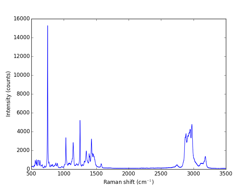
Let us take a look at the raw data.

import numpy as np
import matplotlib.pyplot as plt

w, i = np.loadtxt('data/raman.txt', usecols=(0, 1), unpack=True)

plt.plot(w, i)
plt.xlabel('Raman shift (cm$^{-1}$)')
plt.ylabel('Intensity (counts)')
plt.savefig('images/raman-1.png')
plt.show()
>>> [<matplotlib.lines.Line2D object at 0x10b1d3190>]
<matplotlib.text.Text object at 0x10b1b1b10>
<matplotlib.text.Text object at 0x10bc7f310>

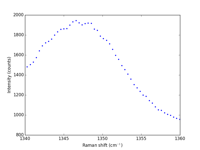
The next thing to do is narrow our focus to the region we are interested in between 1340 cm^{-1} and 1360 cm^{-1}.

ind = (w > 1340) & (w < 1360)
w1 = w[ind]
i1 = i[ind]

plt.plot(w1, i1, 'b. ')
plt.xlabel('Raman shift (cm$^{-1}$)')
plt.ylabel('Intensity (counts)')
plt.savefig('images/raman-2.png')
plt.show()
>>> >>> >>> [<matplotlib.lines.Line2D object at 0x10bc7a4d0>]
<matplotlib.text.Text object at 0x10bc08090>
<matplotlib.text.Text object at 0x10bc49710>

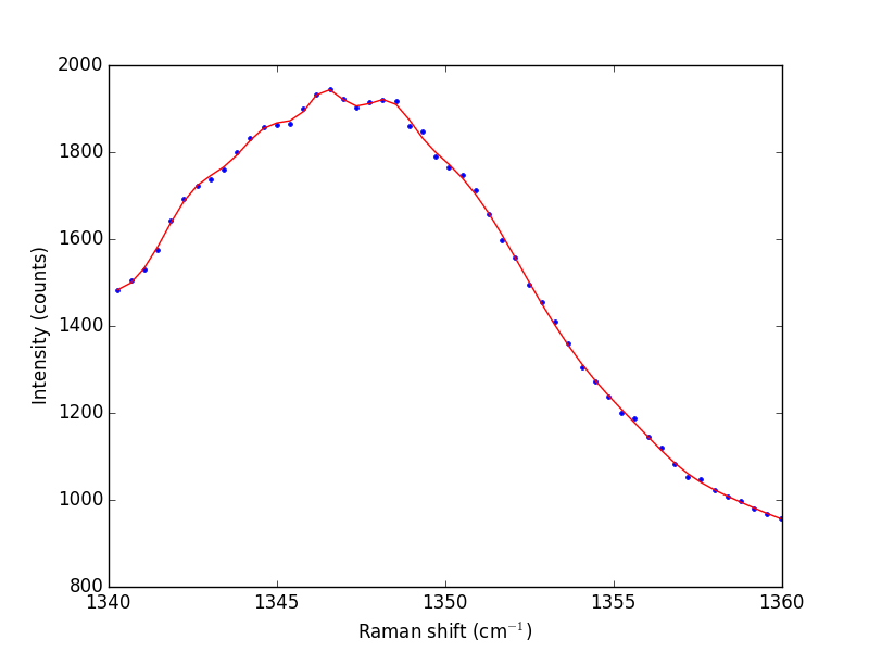
Next we consider a scipy:UnivariateSpline. This function "smooths" the data.

from scipy.interpolate import UnivariateSpline

# s is a "smoothing" factor
sp = UnivariateSpline(w1, i1, k=4, s=2000)

plt.plot(w1, i1, 'b. ')
plt.plot(w1, sp(w1), 'r-')
plt.xlabel('Raman shift (cm$^{-1}$)')
plt.ylabel('Intensity (counts)')
plt.savefig('images/raman-3.png')
plt.show()
>>> ... >>> >>> [<matplotlib.lines.Line2D object at 0x1105633d0>]
[<matplotlib.lines.Line2D object at 0x10dd70250>]
<matplotlib.text.Text object at 0x10dd65f10>
<matplotlib.text.Text object at 0x1105409d0>

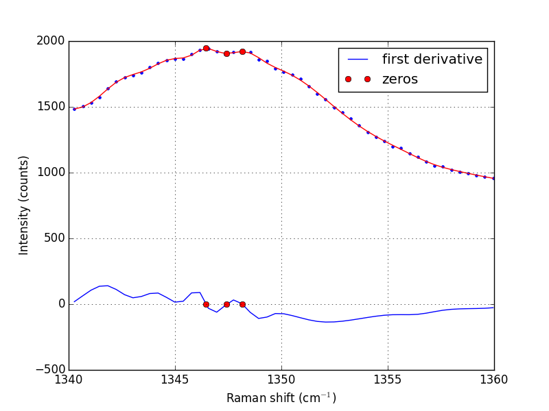
Note that the UnivariateSpline function returns a "callable" function! Our next goal is to find the places where there are peaks. This is defined by the first derivative of the data being equal to zero. It is easy to get the first derivative of a UnivariateSpline with a second argument as shown below.

# get the first derivative evaluated at all the points
d1s = sp.derivative()

d1 = d1s(w1)

# we can get the roots directly here, which correspond to minima and
# maxima.
print('Roots = {}'.format(sp.derivative().roots()))
minmax = sp.derivative().roots()

plt.clf()
plt.plot(w1, d1, label='first derivative')
plt.xlabel('Raman shift (cm$^{-1}$)')
plt.ylabel('First derivative')
plt.grid()

plt.plot(minmax, d1s(minmax), 'ro ', label='zeros')
plt.legend(loc='best')

plt.plot(w1, i1, 'b. ')
plt.plot(w1, sp(w1), 'r-')
plt.xlabel('Raman shift (cm$^{-1}$)')
plt.ylabel('Intensity (counts)')
plt.plot(minmax, sp(minmax), 'ro ')

plt.savefig('images/raman-4.png')
>>> >>> >>> >>> ... ... Roots = [ 1346.4623087   1347.42700893  1348.16689639]
>>> >>> >>> [<matplotlib.lines.Line2D object at 0x1106b2dd0>]
<matplotlib.text.Text object at 0x110623910>
<matplotlib.text.Text object at 0x110c0a090>
>>> >>> [<matplotlib.lines.Line2D object at 0x10b1bacd0>]
<matplotlib.legend.Legend object at 0x1106b2650>
[<matplotlib.lines.Line2D object at 0x1106b2b50>]
[<matplotlib.lines.Line2D object at 0x110698550>]
<matplotlib.text.Text object at 0x110623910>
<matplotlib.text.Text object at 0x110c0a090>
[<matplotlib.lines.Line2D object at 0x110698a10>]

In the end, we have illustrated how to construct a spline smoothing interpolation function and to find maxima in the function, including generating some initial guesses. There is more art to this than you might like, since you have to judge how much smoothing is enough or too much. With too much, you may smooth peaks out. With too little, noise may be mistaken for peaks.

1 Summary notes

Using org-mode with :session allows a large script to be broken up into mini sections. However, it only seems to work with the default python mode in Emacs, and it does not work with emacs-for-python or the latest python-mode. I also do not really like the output style, e.g. the output from the plotting commands.

Copyright (C) 2014 by John Kitchin. See the License for information about copying.

org-mode source

Org-mode version = 8.2.7c

Discuss on Twitter
« Previous Page -- Next Page »