Unique entries in a vector

| categories: python | tags:

Matlab post

It is surprising how often you need to know only the unique entries in a vector of entries. In python, we create a “set” from a list, which only contains unique entries. Then we convert the set back to a list.

a = [1, 1, 2, 3, 4, 5, 3, 5]

b = list(set(a))
print b
[1, 2, 3, 4, 5]
a = ['a',
    'b',
    'abracadabra',
    'b',
    'c',
    'd',
    'b']

print list(set(a))
['a', 'c', 'b', 'abracadabra', 'd']

Copyright (C) 2013 by John Kitchin. See the License for information about copying.

org-mode source
Discuss on Twitter

Constrained optimization

| categories: optimization | tags:

Matlab post

adapted from http://en.wikipedia.org/wiki/Lagrange_multipliers.

Suppose we seek to minimize the function \(f(x,y)=x+y\) subject to the constraint that \(x^2 + y^2 = 1\). The function we seek to maximize is an unbounded plane, while the constraint is a unit circle. We could setup a Lagrange multiplier approach to solving this problem, but we will use a constrained optimization approach instead.

from scipy.optimize import fmin_slsqp

def objective(X):
    x, y = X
    return x + y

def eqc(X):
    'equality constraint'
    x, y = X
    return x**2 + y**2 - 1.0

X0 = [-1, -1]
X = fmin_slsqp(objective, X0, eqcons=[eqc])
print X
Optimization terminated successfully.    (Exit mode 0)
            Current function value: -1.41421356237
            Iterations: 5
            Function evaluations: 20
            Gradient evaluations: 5
[-0.70710678 -0.70710678]

Copyright (C) 2013 by John Kitchin. See the License for information about copying.

org-mode source

Discuss on Twitter

Interpolation with splines

| categories: interpolation | tags:

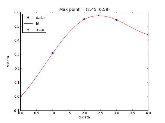
When you do not know the functional form of data to fit an equation, you can still fit/interpolate with splines.

# use splines to fit and interpolate data
from scipy.interpolate import interp1d
from scipy.optimize import fmin
import numpy as np
import matplotlib.pyplot as plt

x = np.array([ 0,      1,      2,      3,      4    ])
y = np.array([ 0.,     0.308,  0.55,   0.546,  0.44 ])

# create the interpolating function
f = interp1d(x, y, kind='cubic', bounds_error=False)

# to find the maximum, we minimize the negative of the function. We
# cannot just multiply f by -1, so we create a new function here.
f2 = interp1d(x, -y, kind='cubic')
xmax = fmin(f2, 2.5)

xfit = np.linspace(0,4)

plt.plot(x,y,'bo')
plt.plot(xfit, f(xfit),'r-')
plt.plot(xmax, f(xmax),'g*')
plt.legend(['data','fit','max'], loc='best', numpoints=1)
plt.xlabel('x data')
plt.ylabel('y data')
plt.title('Max point = ({0:1.2f}, {1:1.2f})'.format(float(xmax),
                                                    float(f(xmax))))
plt.savefig('images/splinefit.png')
Optimization terminated successfully.
         Current function value: -0.575712
         Iterations: 12
         Function evaluations: 24

There are other good examples at http://docs.scipy.org/doc/scipy/reference/tutorial/interpolate.html

Copyright (C) 2013 by John Kitchin. See the License for information about copying.

org-mode source

Discuss on Twitter

Interpolation of data

| categories: interpolation | tags:

Matlab post

When we have data at two points but we need data in between them we use interpolation. Suppose we have the points (4,3) and (6,2) and we want to know the value of y at x=4.65, assuming y varies linearly between these points. we use the interp1d command to achieve this. The syntax in python is slightly different than in matlab.

from scipy.interpolate import interp1d

x = [4, 6]
y = [3, 2]

ifunc = interp1d(x, y)

print ifunc(4.65)


ifunc = interp1d(x, y, bounds_error=False) # do not raise error on out of bounds
print ifunc([4.65, 5.01, 4.2, 9])
2.675
[ 2.675  2.495  2.9      nan]

The default interpolation method is simple linear interpolation between points. Other methods exist too, such as fitting a cubic spline to the data and using the spline representation to interpolate from.

from scipy.interpolate import interp1d

x = [1, 2, 3, 4];
y = [1, 4, 9, 16]; # y = x^2

xi = [ 1.5, 2.5, 3.5]; # we want to interpolate on these values
y1 = interp1d(x,y)

print y1(xi)

y2 = interp1d(x,y,'cubic')
print y2(xi)

import numpy as np
print np.array(xi)**2
[  2.5   6.5  12.5]
[  2.25   6.25  12.25]
[  2.25   6.25  12.25]

In this case the cubic spline interpolation is more accurate than the linear interpolation. That is because the underlying data was polynomial in nature, and a spline is like a polynomial. That may not always be the case, and you need some engineering judgement to know which method is best.

Copyright (C) 2013 by John Kitchin. See the License for information about copying.

org-mode source

Discuss on Twitter

Reading in delimited text files

| categories: io | tags:

Matlab post

sometimes you will get data in a delimited text file format, .e.g. separated by commas or tabs. Matlab can read these in easily. Suppose we have a file containing this data:

1   3
3   4
5   6
4   8

It is easy to read this directly into variables like this:

import numpy as np

x,y = np.loadtxt('data/testdata.txt', unpack=True)

print x,y
[ 1.  3.  5.  4.] [ 3.  4.  6.  8.]

Copyright (C) 2013 by John Kitchin. See the License for information about copying.

org-mode source

Discuss on Twitter
« Previous Page -- Next Page »