A novel way to numerically estimate the derivative of a function - complex-step derivative approximation

| categories: math | tags:

Matlab post

Adapted from http://biomedicalcomputationreview.org/2/3/8.pdf and http://dl.acm.org/citation.cfm?id=838250.838251

This posts introduces a novel way to numerically estimate the derivative of a function that does not involve finite difference schemes. Finite difference schemes are approximations to derivatives that become more and more accurate as the step size goes to zero, except that as the step size approaches the limits of machine accuracy, new errors can appear in the approximated results. In the references above, a new way to compute the derivative is presented that does not rely on differences!

The new way is: \(f'(x) = \rm{imag}(f(x + i\Delta x)/\Delta x)\) where the function \(f\) is evaluated in imaginary space with a small \(\Delta x\) in the complex plane. The derivative is miraculously equal to the imaginary part of the result in the limit of \(\Delta x \rightarrow 0\)!

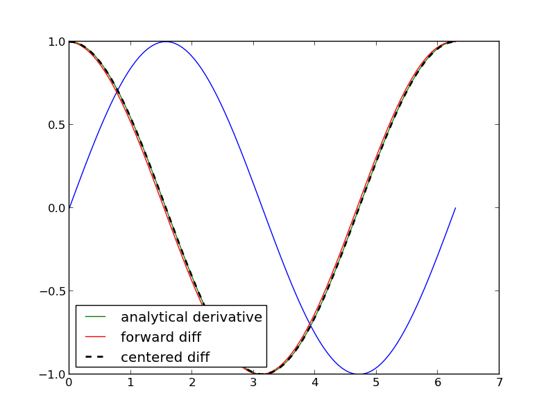
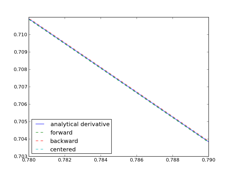
This example comes from the first link. The derivative must be evaluated using the chain rule. We compare a forward difference, central difference and complex-step derivative approximations.

import numpy as np
import matplotlib.pyplot as plt

def f(x):   return np.sin(3*x)*np.log(x)

x = 0.7
h = 1e-7

# analytical derivative
dfdx_a = 3 * np.cos( 3*x)*np.log(x) + np.sin(3*x) / x

# finite difference
dfdx_fd = (f(x + h) - f(x))/h

# central difference
dfdx_cd = (f(x+h)-f(x-h))/(2*h)

# complex method
dfdx_I = np.imag(f(x + np.complex(0, h))/h)

print dfdx_a
print dfdx_fd
print dfdx_cd
print dfdx_cd
1.77335410624
1.7733539398
1.77335410523
1.77335410523

These are all the same to 4 decimal places. The simple finite difference is the least accurate, and the central differences is practically the same as the complex number approach.

Let us use this method to verify the fundamental Theorem of Calculus, i.e. to evaluate the derivative of an integral function. Let \(f(x) = \int\limits_1^{x^2} tan(t^3)dt\), and we now want to compute df/dx. Of course, this can be done analytically, but it is not trivial!

import numpy as np
from scipy.integrate import quad

def f_(z):
    def integrand(t):
        return np.tan(t**3)
    return quad(integrand, 0, z**2)

f = np.vectorize(f_)

x = np.linspace(0, 1)

h = 1e-7

dfdx = np.imag(f(x + complex(0, h)))/h
dfdx_analytical = 2 * x * np.tan(x**6)

import matplotlib.pyplot as plt

plt.plot(x, dfdx, x, dfdx_analytical, 'r--')
plt.show()
>>> >>> ... ... ... ... >>> >>> >>> >>> >>> >>> >>> c:\Python27\lib\site-packages\scipy\integrate\quadpack.py:312: ComplexWarning: Casting complex values to real discards the imaginary part
  return _quadpack._qagse(func,a,b,args,full_output,epsabs,epsrel,limit)
Traceback (most recent call last):
  File "<stdin>", line 1, in <module>
  File "c:\Python27\lib\site-packages\numpy\lib\function_base.py", line 1885, in __call__
    for x, c in zip(self.ufunc(*newargs), self.otypes)])
  File "<stdin>", line 4, in f_
  File "c:\Python27\lib\site-packages\scipy\integrate\quadpack.py", line 247, in quad
    retval = _quad(func,a,b,args,full_output,epsabs,epsrel,limit,points)
  File "c:\Python27\lib\site-packages\scipy\integrate\quadpack.py", line 312, in _quad
    return _quadpack._qagse(func,a,b,args,full_output,epsabs,epsrel,limit)
TypeError: can't convert complex to float
>>> >>> >>> >>> Traceback (most recent call last):
  File "<stdin>", line 1, in <module>
NameError: name 'dfdx' is not defined

Interesting this fails.

Copyright (C) 2013 by John Kitchin. See the License for information about copying.

org-mode source

Discuss on Twitter

Vectorized numeric derivatives

| categories: math | tags:

Loops are usually not great for performance. Numpy offers some vectorized methods that allow us to compute derivatives without loops, although this comes at the mental cost of harder to understand syntax

import numpy as np
import matplotlib.pyplot as plt

x = np.linspace(0, 2 * np.pi, 100)
y = np.sin(x)
dy_analytical = np.cos(x)


# we need to specify the size of dy ahead because diff returns
#an array of n-1 elements
dy = np.zeros(y.shape, np.float) #we know it will be this size
dy[0:-1] = np.diff(y) / np.diff(x)
dy[-1] = (y[-1] - y[-2]) / (x[-1] - x[-2])


'''
calculate dy by center differencing using array slices
'''

dy2 = np.zeros(y.shape,np.float) #we know it will be this size
dy2[1:-1] = (y[2:] - y[0:-2]) / (x[2:] - x[0:-2])

# now the end points
dy2[0] = (y[1] - y[0]) / (x[1] - x[0])
dy2[-1] = (y[-1] - y[-2]) / (x[-1] - x[-2])

plt.plot(x,y)
plt.plot(x,dy_analytical,label='analytical derivative')
plt.plot(x,dy,label='forward diff')
plt.plot(x,dy2,'k--',lw=2,label='centered diff')
plt.legend(loc='lower left')
plt.savefig('images/vectorized-diffs.png')
plt.show()

Copyright (C) 2013 by John Kitchin. See the License for information about copying.

org-mode source

Discuss on Twitter

Numeric derivatives by differences

| categories: math | tags:

numpy has a function called numpy.diff() that is similar to the one found in matlab. It calculates the differences between the elements in your list, and returns a list that is one element shorter, which makes it unsuitable for plotting the derivative of a function.

Loops in python are pretty slow (relatively speaking) but they are usually trivial to understand. In this script we show some simple ways to construct derivative vectors using loops. It is implied in these formulas that the data points are equally spaced. If they are not evenly spaced, you need a different approach.

import numpy as np
from pylab import *
import time

'''
These are the brainless way to calculate numerical derivatives. They
work well for very smooth data. they are surprisingly fast even up to
10000 points in the vector.
'''

x = np.linspace(0.78,0.79,100)
y = np.sin(x)
dy_analytical = np.cos(x)
'''
lets use a forward difference method:
that works up until the last point, where there is not
a forward difference to use. there, we use a backward difference.
'''

tf1 = time.time()
dyf = [0.0]*len(x)
for i in range(len(y)-1):
    dyf[i] = (y[i+1] - y[i])/(x[i+1]-x[i])
#set last element by backwards difference
dyf[-1] = (y[-1] - y[-2])/(x[-1] - x[-2])

print ' Forward difference took %1.1f seconds' % (time.time() - tf1)

'''and now a backwards difference'''
tb1 = time.time()
dyb = [0.0]*len(x)
#set first element by forward difference
dyb[0] = (y[0] - y[1])/(x[0] - x[1])
for i in range(1,len(y)):
    dyb[i] = (y[i] - y[i-1])/(x[i]-x[i-1])

print ' Backward difference took %1.1f seconds' % (time.time() - tb1)

'''and now, a centered formula'''
tc1 = time.time()
dyc = [0.0]*len(x)
dyc[0] = (y[0] - y[1])/(x[0] - x[1])
for i in range(1,len(y)-1):
    dyc[i] = (y[i+1] - y[i-1])/(x[i+1]-x[i-1])
dyc[-1] = (y[-1] - y[-2])/(x[-1] - x[-2])

print ' Centered difference took %1.1f seconds' % (time.time() - tc1)

'''
the centered formula is the most accurate formula here
'''

plt.plot(x,dy_analytical,label='analytical derivative')
plt.plot(x,dyf,'--',label='forward')
plt.plot(x,dyb,'--',label='backward')
plt.plot(x,dyc,'--',label='centered')

plt.legend(loc='lower left')
plt.savefig('images/simple-diffs.png')
plt.show()
Forward difference took 0.0 seconds
Backward difference took 0.0 seconds
Centered difference took 0.0 seconds

Copyright (C) 2013 by John Kitchin. See the License for information about copying.

org-mode source

Discuss on Twitter

Indexing vectors and arrays in Python

| categories: basic | tags:

Matlab post There are times where you have a lot of data in a vector or array and you want to extract a portion of the data for some analysis. For example, maybe you want to plot column 1 vs column 2, or you want the integral of data between x = 4 and x = 6, but your vector covers 0 < x < 10. Indexing is the way to do these things.

A key point to remember is that in python array/vector indices start at 0. Unlike Matlab, which uses parentheses to index a array, we use brackets in python.

import numpy as np

x = np.linspace(-np.pi, np.pi, 10)
print x

print x[0]  # first element
print x[2]  # third element
print x[-1] # last element
print x[-2] # second to last element
>>> >>> [-3.14159265 -2.44346095 -1.74532925 -1.04719755 -0.34906585  0.34906585
  1.04719755  1.74532925  2.44346095  3.14159265]
>>> -3.14159265359
-1.74532925199
3.14159265359
2.44346095279

We can select a range of elements too. The syntax a:b extracts the a^{th} to (b-1)^{th} elements. The syntax a:b:n starts at a, skips nelements up to the index b.

print x[1:4]     # second to fourth element. Element 5 is not included
print x[0:-1:2]  # every other element
print x[:]       # print the whole vector
print x[-1:0:-1] # reverse the vector!
[-2.44346095 -1.74532925 -1.04719755]
[-3.14159265 -1.74532925 -0.34906585  1.04719755  2.44346095]
[-3.14159265 -2.44346095 -1.74532925 -1.04719755 -0.34906585  0.34906585
  1.04719755  1.74532925  2.44346095  3.14159265]
[ 3.14159265  2.44346095  1.74532925  1.04719755  0.34906585 -0.34906585
 -1.04719755 -1.74532925 -2.44346095]

Suppose we want the part of the vector where x > 2. We could do that by inspection, but there is a better way. We can create a mask of boolean (0 or 1) values that specify whether x > 2 or not, and then use the mask as an index.

print x[x > 2]
[ 2.44346095  3.14159265]

You can use this to analyze subsections of data, for example to integrate the function y = sin(x) where x > 2.

y = np.sin(x)

print np.trapz( x[x > 2], y[x > 2])
>>> -1.79500162881

1 2d arrays

In 2d arrays, we use row, column notation. We use a : to indicate all rows or all columns.

a = np.array([[1, 2, 3], 
              [4, 5, 6], 
              [7, 8, 9]])

print a[0, 0]
print a[-1, -1]

print a[0, :] # row one
print a[:, 0] # column one
print a[:]
... >>> >>> 1
9
>>> [1 2 3]
[1 4 7]
[[1 2 3]
 [4 5 6]
 [7 8 9]]

2 Using indexing to assign values to rows and columns

b = np.zeros((3, 3))
print b

b[:, 0] = [1, 2, 3] # set column 0
b[2, 2] = 12        # set a single element
print b

b[2] = 6  # sets everything in row 2 to 6!
print b
[[ 0.  0.  0.]
 [ 0.  0.  0.]
 [ 0.  0.  0.]]
>>> >>> >>> [[  1.   0.   0.]
 [  2.   0.   0.]
 [  3.   0.  12.]]
>>> >>> [[ 1.  0.  0.]
 [ 2.  0.  0.]
 [ 6.  6.  6.]]

Python does not have the linear assignment method like Matlab does. You can achieve something like that as follows. We flatten the array to 1D, do the linear assignment, and reshape the result back to the 2D array.

c = b.flatten()
c[2] = 34
b[:] = c.reshape(b.shape)
print b
>>> >>> [[  1.   0.  34.]
 [  2.   0.   0.]
 [  6.   6.   6.]]

3 3D arrays

The 3d array is like book of 2D matrices. Each page has a 2D matrix on it. think about the indexing like this: (row, column, page)

M = np.random.uniform(size=(3,3,3))  # a 3x3x3 array
print M
[[[ 0.78557795  0.36454381  0.96090072]
  [ 0.76133373  0.03250485  0.08517174]
  [ 0.96007909  0.08654002  0.29693648]]

 [[ 0.58270738  0.60656083  0.47703339]
  [ 0.62551477  0.62244626  0.11030327]
  [ 0.2048839   0.83081982  0.83660668]]

 [[ 0.12489176  0.20783996  0.38481792]
  [ 0.05234762  0.03989146  0.09731516]
  [ 0.67427208  0.51793637  0.89016255]]]
print M[:, :, 0]  # 2d array on page 0
print M[:, 0, 0]  # column 0 on page 0
print M[1, :, 2]  # row 1 on page 2
[[ 0.78557795  0.76133373  0.96007909]
 [ 0.58270738  0.62551477  0.2048839 ]
 [ 0.12489176  0.05234762  0.67427208]]
[ 0.78557795  0.58270738  0.12489176]
[ 0.47703339  0.11030327  0.83660668]

4 Summary

The most common place to use indexing is probably when a function returns an array with the independent variable in column 1 and solution in column 2, and you want to plot the solution. Second is when you want to analyze one part of the solution. There are also applications in numerical methods, for example in assigning values to the elements of a matrix or vector.

Copyright (C) 2013 by John Kitchin. See the License for information about copying.

org-mode source

Discuss on Twitter

Advanced function creation

| categories: python | tags:

Python has some nice features in creating functions. You can create default values for variables, have optional variables and optional keyword variables. In this function f(a,b), a and b are called positional arguments, and they are required, and must be provided in the same order as the function defines.

If we provide a default value for an argument, then the argument is called a keyword argument, and it becomes optional. You can combine positional arguments and keyword arguments, but positional arguments must come first. Here is an example.

def func(a, n=2):
    "compute the nth power of a"
    return a**n

# three different ways to call the function
print func(2)
print func(2, 3)
print func(2, n=4)
4
8
16

In the first call to the function, we only define the argument a, which is a mandatory, positional argument. In the second call, we define a and n, in the order they are defined in the function. Finally, in the third call, we define a as a positional argument, and n as a keyword argument.

If all of the arguments are optional, we can even call the function with no arguments. If you give arguments as positional arguments, they are used in the order defined in the function. If you use keyword arguments, the order is arbitrary.

def func(a=1, n=2):
    "compute the nth power of a"
    return a**n

# three different ways to call the function
print func()
print func(2, 4)
print func(n=4, a=2)
1
16
16

It is occasionally useful to allow an arbitrary number of arguments in a function. Suppose we want a function that can take an arbitrary number of positional arguments and return the sum of all the arguments. We use the syntax *args to indicate arbitrary positional arguments. Inside the function the variable args is a tuple containing all of the arguments passed to the function.

def func(*args):
    sum = 0
    for arg in args:
        sum += arg
    return sum

print func(1, 2, 3, 4)
10

A more “functional programming” version of the last function is given here. This is an advanced approach that is less readable to new users, but more compact and likely more efficient for large numbers of arguments.

import operator
def func(*args):
    return reduce(operator.add, args)
print func(1, 2, 3, 4)
10

It is possible to have arbitrary keyword arguments. This is a common pattern when you call another function within your function that takes keyword arguments. We use **kwargs to indicate that arbitrary keyword arguments can be given to the function. Inside the function, kwargs is variable containing a dictionary of the keywords and values passed in.

def func(**kwargs):
    for kw in kwargs:
        print '{0} = {1}'.format(kw, kwargs[kw])

func(t1=6, color='blue')
color = blue
t1 = 6

A typical example might be:

import matplotlib.pyplot as plt

def myplot(x, y, fname=None, **kwargs):
    "make plot of x,y. save to fname if not None. provide kwargs to plot"
    plt.plot(x, y, **kwargs)
    plt.xlabel('X')
    plt.ylabel('Y')
    plt.title('My plot')
    if fname:
        plt.savefig(fname)
    else:
        plt.show()

x = [1, 3, 4, 5]
y = [3, 6, 9, 12]

myplot(x, y, 'images/myfig.png', color='orange', marker='s')

# you can use a dictionary as kwargs
d = {'color':'magenta',
     'marker':'d'}

myplot(x, y, 'images/myfig2.png', **d)

In that example we wrap the matplotlib plotting commands in a function, which we can call the way we want to, with arbitrary optional arguments. In this example, you cannot pass keyword arguments that are illegal to the plot command or you will get an error.

It is possible to combine all the options at once. I admit it is hard to imagine where this would be really useful, but it can be done!

import numpy as np

def func(a, b=2, *args, **kwargs):
    "return a**b + sum(args) and print kwargs"
    for kw in kwargs:
        print 'kw: {0} = {1}'.format(kw, kwargs[kw])

    return a**b + np.sum(args)

print func(2, 3, 4, 5, mysillykw='hahah')
kw: mysillykw = hahah
17

Copyright (C) 2013 by John Kitchin. See the License for information about copying.

org-mode source

Discuss on Twitter
« Previous Page -- Next Page »