Notice anything different

| categories: uncategorized | tags:

Based on the last few posts on making links to external files work in the blog, and customizing code block export in HTML, I have rewritten blogofile.elto more cleanly support the use of images and data files in my blog posts. Now, I should be able to include a data file (like this one) in a post and you should be able to click on the link to open it after I publish the post in the usual way by pressing F10. That should process the post, construct URLs for all the links, including images, copy the relevant files to the blog directory, and generate the HTML file for blogofile to build. This is a little more robust than it used to be, as all files are stored in a directory named based on the post title, so there is less concern of using duplicate filenames for images and datafiles.

Here is a gratuitous image, just to see if it works ;)
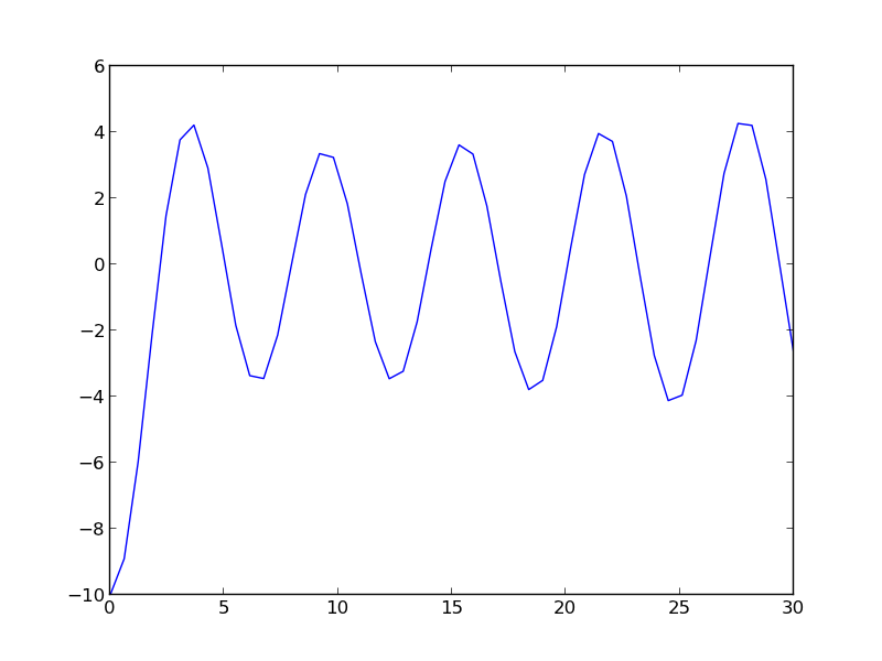
Figure 1: test image

Hopefully, there is nothing different on the outside! URLs to images are now in a different place, but that should not be apparent unless you read source code. The real difference is that now there are working links to data files! And it is easier for me to write my posts including them, with simple publishing.

Copyright (C) 2013 by John Kitchin. See the License for information about copying.
org-mode source

Discuss on Twitter

Estimating uncertainties in equations of state

| categories: uncategorized | tags:

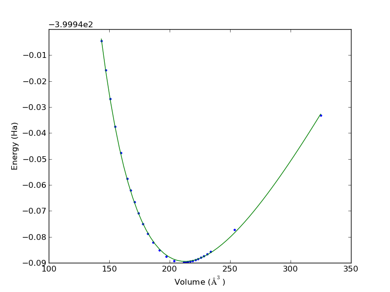
We often use DFT to calculate the energy of a unit cell as a function of volume. Then, we fit an equation of state to the data to estimate the volume that minimizes the total energy, and the bulk modulus of the material. 10.1016/j.comphys.2003.12.001

volume energy
324.85990899 -399.9731688470
253.43999457 -400.0172393178
234.03826687 -400.0256270548
231.12159387 -400.0265690700
228.40609504 -400.0273551120
225.86490337 -400.0280030862
223.47556626 -400.0285313450
221.21992353 -400.0289534593
219.08319566 -400.0292800709
217.05369547 -400.0295224970
215.12089909 -400.0296863867
213.27525144 -400.0297809256
211.51060823 -400.0298110000
203.66743321 -400.0291665573
197.07888649 -400.0275017142
191.39717952 -400.0250998136
186.40163591 -400.0221371852
181.94435510 -400.0187369863
177.92077043 -400.0149820198
174.25380090 -400.0109367042
170.88582166 -400.0066495100
167.76711189 -400.0021478258
164.87096104 -399.9974753449
159.62553397 -399.9876885136
154.97005460 -399.9774175487
150.78475335 -399.9667603369
146.97722201 -399.9557686286
143.49380641 -399.9445262604
import numpy as np
import matplotlib.pyplot as plt
from pycse import nlinfit

# data
V = np.array([row[0] for row in data]) 
E = np.array([row[1] for row in data])

plt.plot(V, E, '.')
plt.xlabel('Volume ($\AA^3$)')
plt.ylabel('Energy (Ha)')

def Murnaghan(vol, E0, B0, BP, V0):
    '''
    given a vector of parameters and volumes, return a vector of energies.
    equation From PRB 28,5480 (1983)
    '''
    
    E = E0 + B0*vol/BP*(((V0/vol)**BP)/(BP-1)+1) - V0*B0/(BP-1.)

    return E

guess = [-400, 0.5, 2, 210]
pars, pint, SE = nlinfit(Murnaghan, V, E, guess, alpha=0.05)
E0, B0, BP, V0 = pint

Vfit = np.linspace(V.min(), V.max())
plt.plot(Vfit, Murnaghan(Vfit, *pars))
plt.savefig('images/eos-uncertainty.png')

print '95% confidence intervals'
print 'V0 = {0} bohr**3'.format(V0)
print 'E0 = {0} Ha'.format(E0)
print 'B0 = {0} GPA'.format([x * 29421.010901602753 for x in B0])
95% confidence intervals
V0 = [212.27788154532402, 213.27897592511891] bohr**3
E0 = [-400.0297027767362, -400.02922937100408] Ha
B0 = [108.62283904402159, 111.20447706313001] GPA

You can see the fit is not perfect, and there is corresponding uncertainty in the estimated parameters. A nice feature of the Murnaghan equation of state is that the parameters are directly the quantities of interest, so the uncertainties are directly calculated here. For other models, e.g. a polynomial fit, you would have to propagate the errors in the parameters to the properties.

Copyright (C) 2013 by John Kitchin. See the License for information about copying.
org-mode source

Discuss on Twitter

Finding the volume of a unit cell at a fixed pressure

| categories: uncategorized | tags:

A typical unit cell optimization in DFT is performed by minimizing the total energy with respect to variations in the unit cell parameters and atomic positions. In this approach, a pressure of 0 GPa is implied, as well as a temperature of 0K. For non-zero pressures, the volume that minimizes the total energy is not the same as the volume at P=0.

Let \(x\) be the unit cell parameters that can be varied. For P ≠ 0, and T = 0, we have the following

\(G(x; p) = E(x) + p V(x)\)

and we need to minimize this function to find the groundstate volume. We will do this for fcc Cu at 5 GPa of pressure. We will assume there is only one degree of freedom in the unit cell, the lattice constant. First we get the \(E(x)\) function, and then add the analytical correction.

from jasp import *
from ase import Atom, Atoms
from ase.utils.eos import EquationOfState

LC = [3.5, 3.55, 3.6, 3.65, 3.7, 3.75]
volumes, energies = [], []
ready = True

P = 5.0 / 160.2176487  # pressure in eV/ang**3

for a in LC:
    atoms = Atoms([Atom('Cu',(0, 0, 0))],
              cell=0.5 * a*np.array([[1.0, 1.0, 0.0],
                                     [0.0, 1.0, 1.0],
                                     [1.0, 0.0, 1.0]]))

    with jasp('../bulk/Cu-{0}'.format(a),
              xc='PBE',
              encut=350,
              kpts=(8,8,8),
              atoms=atoms) as calc:

        try:
            e = atoms.get_potential_energy()
            energies.append(e)
            volumes.append(atoms.get_volume())
        except (VaspSubmitted, VaspQueued):
            ready = False

if not ready:
    import sys; sys.exit()

import numpy as np
energies = np.array(energies)
volumes = np.array(volumes)

eos = EquationOfState(volumes, energies)
v0, e0, B = eos.fit()
print 'V0 at 0 GPa = {0:1.2f} ang^3'.format(v0)

eos5 = EquationOfState(volumes, energies + P * volumes)
v0_5, e0, B = eos5.fit()
print 'V0 at 5 GPa = {0:1.2f} ang^3'.format(v0_5)
V0 at 0 GPa = 12.02 ang^3
V0 at 5 GPa = 11.62 ang^3

You can see here that apply pressure decreases the equilibrium volume, and increases the total energy.

Copyright (C) 2013 by John Kitchin. See the License for information about copying.
org-mode source

Discuss on Twitter

Meet the steam tables

| categories: uncategorized | tags: steam, thermodynamics

Matlab post

We will use the iapws module. Install it like this:

pip install iapws

Problem statement: A Rankine cycle operates using steam with the condenser at 100 degC, a pressure of 3.0 MPa and temperature of 600 degC in the boiler. Assuming the compressor and turbine operate reversibly, estimate the efficiency of the cycle.

Starting point in the Rankine cycle in condenser.

we have saturated liquid here, and we get the thermodynamic properties for the given temperature. In this python module, these properties are all in attributes of an IAPWS object created at a set of conditions.

1 Starting point in the Rankine cycle in condenser.

We have saturated liquid here, and we get the thermodynamic properties for the given temperature.

from iapws import IAPWS97

T1 = 100 + 273.15 #in K

sat_liquid1  = IAPWS97(T=T1, x=0) # x is the steam quality. 0 = liquid

P1 = sat_liquid1.P
s1 = sat_liquid1.s
h1 = sat_liquid1.h
v1 = sat_liquid1.v

2 Isentropic compression of liquid to point 2

The final pressure is given, and we need to compute the new temperatures, and enthalpy.

P2 = 3.0 # MPa
s2 = s1 # this is what isentropic means

sat_liquid2 = IAPWS97(P=P2, s=s1)
T2, = sat_liquid2.T
h2 = sat_liquid2.h

# work done to compress liquid. This is an approximation, since the
# volume does change a little with pressure, but the overall work here
# is pretty small so we neglect the volume change.
WdotP = v1*(P2 - P1);
print
print('The compressor work is: {0:1.4f} kJ/kg'.format(WdotP))
>>> >>> >>> >>> >>> >>> ... ... ... >>>
The compressor work is: 0.0030 kJ/kg

The compression work is almost negligible. This number is 1000 times smaller than we computed with Xsteam. I wonder what the units of v1 actually are.

3 Isobaric heating to T3 in boiler where we make steam

T3 = 600 + 273.15 # K
P3 = P2 # definition of isobaric
steam = IAPWS97(P=P3, T=T3)

h3 = steam.h
s3 = steam.s

Qb, = h3 - h2 # heat required to make the steam

print
print 'The boiler heat duty is: {0:1.2f} kJ/kg'.format(Qb)
>>> >>> >>> >>> >>> >>> >>> >>>
The boiler heat duty is: 3260.69 kJ/kg

4 Isentropic expansion through turbine to point 4

steam =  IAPWS97(P=P1, s=s3)
T4, = steam.T
h4 = steam.h
s4 = s3 # isentropic
Qc, = h4 - h1 # work required to cool from T4 to T1
print 
print 'The condenser heat duty is {0:1.2f} kJ/kg'.format(Qc)
>>> >>> >>> >>>
The condenser heat duty is 2317.00 kJ/kg

5 To get from point 4 to point 1

WdotTurbine, = h4 - h3 # work extracted from the expansion
print('The turbine work is: {0:1.2f} kJ/kg'.format(WdotTurbine))
The turbine work is: -946.71 kJ/kg

6 Efficiency

This is a ratio of the work put in to make the steam, and the net work obtained from the turbine. The answer here agrees with the efficiency calculated in Sandler on page 135.

eta = -(WdotTurbine - WdotP) / Qb
print('The overall efficiency is {0:1.2%}.'.format(eta))
The overall efficiency is 29.03%.

7 Entropy-temperature chart

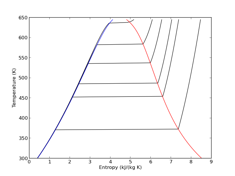
The IAPWS module makes it pretty easy to generate figures of the steam tables. Here we generate an entropy-Temperature graph. We do this to illustrate the path of the Rankine cycle. We need to compute the values of steam entropy for a range of pressures and temperatures.

import numpy as np
import matplotlib.pyplot as plt

plt.figure()
plt.clf()
T = np.linspace(300, 372+273, 200) # range of temperatures
for P in [0.1, 1, 2, 5, 10, 20]: #MPa
    steam = [IAPWS97(T=t, P=P) for t in T]
    S = [s.s for s in steam]
    plt.plot(S, T, 'k-')

# saturated vapor and liquid entropy lines
svap = [s.s for s in [IAPWS97(T=t, x=1) for t in T]]
sliq = [s.s for s in [IAPWS97(T=t, x=0) for t in T]]

plt.plot(svap, T, 'r-')
plt.plot(sliq, T, 'b-')

plt.xlabel('Entropy (kJ/(kg K)')
plt.ylabel('Temperature (K)')
plt.savefig('images/iawps-steam.png')
>>> >>> <matplotlib.figure.Figure object at 0x000000000638BC18>
>>> >>> ... ... ... ... [<matplotlib.lines.Line2D object at 0x0000000007F9C208>]
[<matplotlib.lines.Line2D object at 0x0000000007F9C400>]
[<matplotlib.lines.Line2D object at 0x0000000007F9C8D0>]
[<matplotlib.lines.Line2D object at 0x0000000007F9CD30>]
[<matplotlib.lines.Line2D object at 0x0000000007F9E1D0>]
[<matplotlib.lines.Line2D object at 0x0000000007F9E630>]
... >>> >>> >>> [<matplotlib.lines.Line2D object at 0x0000000001FDCEB8>]
[<matplotlib.lines.Line2D object at 0x0000000007F9EA90>]
>>> <matplotlib.text.Text object at 0x0000000007F7BE48>
<matplotlib.text.Text object at 0x0000000007F855F8>

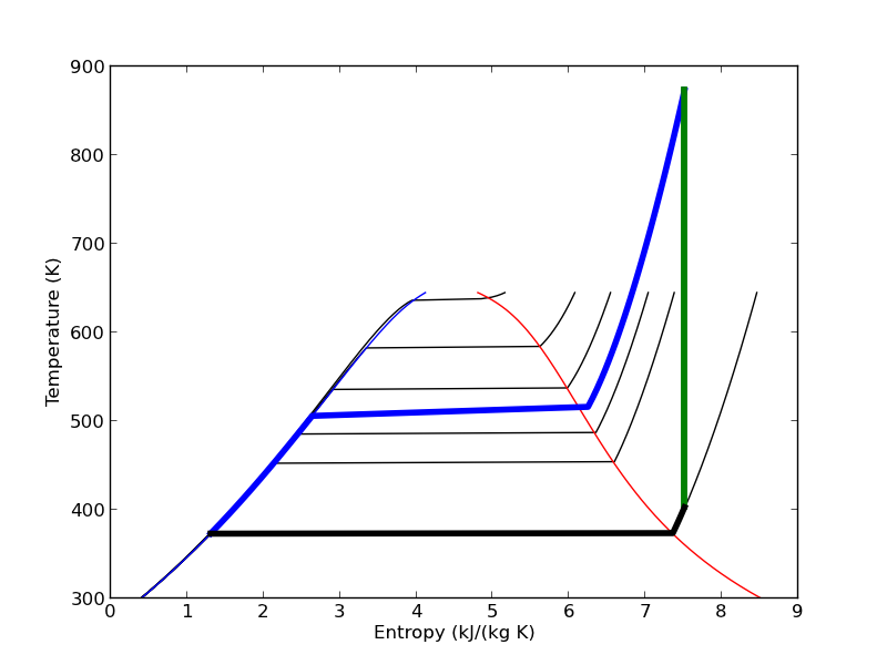
We can plot our Rankine cycle path like this. We compute the entropies along the non-isentropic paths.

T23 = np.linspace(T2, T3)
S23 = [s.s for s in [IAPWS97(P=P2, T=t) for t in T23]]

T41 = np.linspace(T4, T1 - 0.01) # subtract a tiny bit to make sure we get a liquid
S41 = [s.s for s in [IAPWS97(P=P1, T=t) for t in T41]]

And then we plot the paths.

plt.plot([s1, s2], [T1, T2], 'r-', lw=4) # Path 1 to 2
plt.plot(S23, T23, 'b-', lw=4) # path from 2 to 3 is isobaric
plt.plot([s3, s4], [T3, T4], 'g-', lw=4) # path from 3 to 4 is isentropic
plt.plot(S41, T41, 'k-', lw=4) # and from 4 to 1 is isobaric
plt.savefig('images/iawps-steam-2.png')
plt.savefig('images/iawps-steam-2.svg')
[<matplotlib.lines.Line2D object at 0x0000000008350908>]
[<matplotlib.lines.Line2D object at 0x00000000083358D0>]
[<matplotlib.lines.Line2D object at 0x000000000835BEB8>]
[<matplotlib.lines.Line2D object at 0x0000000008357160>]

8 Summary

This was an interesting exercise. On one hand, the tedium of interpolating the steam tables is gone. On the other hand, you still have to know exactly what to ask for to get an answer that is correct. The iapws interface is a little clunky, and takes some getting used to. It does not seem as robust as the Xsteam module I used in Matlab.

Copyright (C) 2013 by John Kitchin. See the License for information about copying.
org-mode source

Discuss on Twitter

Estimating the boiling point of water

| categories: uncategorized | tags: thermodynamics

Matlab post

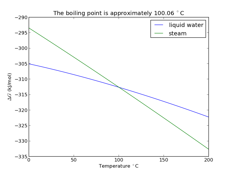
I got distracted looking for Shomate parameters for ethane today, and came across this website on predicting the boiling point of water using the Shomate equations. The basic idea is to find the temperature where the Gibbs energy of water as a vapor is equal to the Gibbs energy of the liquid.

import matplotlib.pyplot as plt

Liquid water (\url{http://webbook.nist.gov/cgi/cbook.cgi?ID=C7732185&Units=SI&Mask=2#Thermo-Condensed})

# valid over 298-500

Hf_liq = -285.830   # kJ/mol
S_liq = 0.06995     # kJ/mol/K
shomateL = [-203.6060,
            1523.290,
           -3196.413,
            2474.455,
               3.855326,
            -256.5478,
            -488.7163,
            -285.8304]

Gas phase water (\url{http://webbook.nist.gov/cgi/cbook.cgi?ID=C7732185&Units=SI&Mask=1&Type=JANAFG&Table=on#JANAFG})

Interestingly, these parameters are listed as valid only above 500K. That means we have to extrapolate the values down to 298K. That is risky for polynomial models, as they can deviate substantially outside the region they were fitted to.

Hf_gas = -241.826  # kJ/mol
S_gas = 0.188835   # kJ/mol/K

shomateG = [30.09200,
             6.832514,
             6.793435,
            -2.534480,
             0.082139,
          -250.8810,
           223.3967,
          -241.8264]

Now, we wan to compute G for each phase as a function of T

import numpy as np

T = np.linspace(0, 200) + 273.15
t = T / 1000.0

sTT = np.vstack([np.log(t),
                 t,
                 (t**2) / 2.0,
                 (t**3) / 3.0,
                 -1.0 / (2*t**2),
                 0 * t,
                 t**0,
                 0 * t**0]).T / 1000.0

hTT = np.vstack([t,
                 (t**2)/2.0,
                 (t**3)/3.0,
                 (t**4)/4.0,
                 -1.0 / t,
                 1 * t**0,
                 0 * t**0,
                 -1 * t**0]).T

Gliq = Hf_liq + np.dot(hTT, shomateL) - T*(np.dot(sTT, shomateL))
Ggas = Hf_gas + np.dot(hTT, shomateG) - T*(np.dot(sTT, shomateG))
                 
from scipy.interpolate import interp1d
from scipy.optimize import fsolve

f = interp1d(T, Gliq - Ggas)
bp, = fsolve(f, 373)
print 'The boiling point is {0} K'.format(bp)
>>> >>> >>> >>> ... ... ... ... ... ... ... >>> >>> ... ... ... ... ... ... ... >>> >>> >>> >>> ... >>> >>> >>> >>> >>> The boiling point is 373.206081312 K
plt.figure(); plt.clf()
plt.plot(T-273.15, Gliq, T-273.15, Ggas)
plt.legend(['liquid water', 'steam'])

plt.xlabel('Temperature $^\circ$C')
plt.ylabel('$\Delta G$ (kJ/mol)')
plt.title('The boiling point is approximately {0:1.2f} $^\circ$C'.format(bp-273.15))
plt.savefig('images/boiling-water.png')
<matplotlib.figure.Figure object at 0x050D2E30>
[<matplotlib.lines.Line2D object at 0x051AB610>, <matplotlib.lines.Line2D object at 0x051B4C90>]
<matplotlib.legend.Legend object at 0x051B9030>
>>> <matplotlib.text.Text object at 0x0519E390>
<matplotlib.text.Text object at 0x050FB390>
<matplotlib.text.Text object at 0x050FBFB0>

1 Summary

The answer we get us 0.05 K too high, which is not bad considering we estimated it using parameters that were fitted to thermodynamic data and that had finite precision and extrapolated the steam properties below the region the parameters were stated to be valid for.

Copyright (C) 2013 by John Kitchin. See the License for information about copying.

org-mode source

Discuss on Twitter
« Previous Page