Modeling a Cu dimer by EMT, nonlinear regression and neural networks

| categories: machine-learning, molecular-simulation, neural-network, python | tags:

In this post we consider a Cu2 dimer and how its energy varies with the separation of the atoms. We assume we have a way to calculate this, but that it is expensive, and that we want to create a simpler model that is as accurate, but cheaper to run. A simple way to do that is to regress a physical model, but we will illustrate some challenges with that. We then show a neural network can be used as an accurate regression function without needing to know more about the physics.

We will use an effective medium theory calculator to demonstrate this. The calculations are not expected to be very accurate or relevant to any experimental data, but they are fast, and will illustrate several useful points that are independent of that. We will take as our energy zero the energy of two atoms at a large separation, in this case about 10 angstroms. Here we plot the energy as a function of the distance between the two atoms, which is the only degree of freedom that matters in this example.

import numpy as np
%matplotlib inline
import matplotlib.pyplot as plt

from ase.calculators.emt import EMT
from ase import Atoms

atoms = Atoms('Cu2',[[0, 0, 0], [10, 0, 0]], pbc=[False, False, False])
atoms.set_calculator(EMT())

e0 = atoms.get_potential_energy()

# Array of bond lengths to get the energy for
d = np.linspace(1.7, 3, 30)

def get_e(distance):
    a = atoms.copy()
    a[1].x = distance
    a.set_calculator(EMT())
    e = a.get_potential_energy()
    return e

e = np.array([get_e(dist) for dist in d])
e -=  e0  # set the energy zero

plt.plot(d, e, 'bo ')
plt.xlabel('d (Å)')
plt.ylabel('energy (eV)')
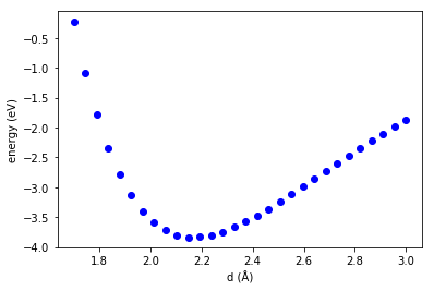
We see there is a minimum, and the energy is asymmetric about the minimum. We have no functional form for the energy here, just the data in the plot. So to get another energy, we have to run another calculation. If that was expensive, we might prefer an analytical equation to evaluate instead. We will get an analytical form by fitting a function to the data. A classic one is the Buckingham potential: \(E = A \exp(-B r) - \frac{C}{r^6}\). Here we perform the regression.

def model(r, A, B, C):
    return A * np.exp(-B * r) - C / r**6

from pycse import nlinfit
import pprint

p0 = [-80, 1, 1]
p, pint, se = nlinfit(model, d, e, p0, 0.05)
print('Parameters = ', p)
print('Confidence intervals = ')
pprint.pprint(pint)
plt.plot(d, e, 'bo ', label='calculations')

x = np.linspace(min(d), max(d))
plt.plot(x, model(x, *p), label='fit')
plt.legend(loc='best')
plt.xlabel('d (Å)')
plt.ylabel('energy (eV)')

Parameters = [ -83.21072545 1.18663393 -266.15259507] Confidence intervals = array([[ -93.47624687, -72.94520404], [ 1.14158438, 1.23168348], [-280.92915682, -251.37603331]])
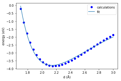
That fit is ok, but not great. We would be better off with a spline for this simple system! The trouble is how do we get anything better? If we had a better equation to fit to we might get better results. While one might come up with one for this dimer, how would you extend it to more complex systems, even just a trimer? There have been decades of research dedicated to that, and we are not smarter than those researchers so, it is time for a new approach.

We will use a Neural Network regressor. The input will be \(d\) and we want to regress a function to predict the energy.

There are a couple of important points to make here.

  1. This is just another kind of regression.
  2. We need a lot more data to do the regression. Here we use 300 data points.
  3. We need to specify a network architecture. Here we use one hidden layer with 10 neurons, and the tanh activation function on each neuron. The last layer is just the output layer. I do not claim this is any kind of optimal architecture. It is just one that works to illustrate the idea.

Here is the code that uses a neural network regressor, which is lightly adapted from http://scikit-neuralnetwork.readthedocs.io/en/latest/guide_model.html.

from sknn.mlp import Regressor, Layer

D = np.linspace(1.7, 3, 300)

def get_e(distance):
    a = atoms.copy()
    a[1].x = distance
    a.set_calculator(EMT())
    e = a.get_potential_energy()
    return e

E = np.array([get_e(dist) for dist in D])
E -=  e0  # set the energy zero

X_train = np.row_stack(np.array(D))

N = 10
nn = Regressor(layers=[Layer("Tanh", units=N),
                       Layer('Linear')])
nn.fit(X_train, E)

dfit = np.linspace(min(d), max(d))

efit = nn.predict(np.row_stack(dfit))

plt.plot(d, e, 'bo ')
plt.plot(dfit, efit)
plt.legend(['calculations', 'neural network'])
plt.xlabel('d (Å)')
plt.ylabel('energy (eV)')
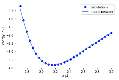
This fit looks pretty good, better than we got for the Buckingham potential. Well, it probably should look better, we have many more parameters that were fitted! It is not perfect, but it could be systematically improved by increasing the number of hidden layers, and neurons in each layer. I am being a little loose here by relying on a visual assessment of the fit. To systematically improve it you would need a quantitative analysis of the errors. I also note though, that if I run the block above several times in succession, I get different fits each time. I suppose that is due to some random numbers used to initialize the fit, but sometimes the fit is about as good as the result you see above, and sometimes it is terrible.

Ok, what is the point after all? We developed a neural network that pretty accurately captures the energy of a Cu dimer with no knowledge of the physics involved. Now, EMT is not that expensive, but suppose this required 300 DFT calculations at 1 minute or more a piece? That is five hours just to get the data! With this neural network, we can quickly compute energies. For example, this shows we get about 10000 energy calculations in just 287 ms.

%%timeit

dfit = np.linspace(min(d), max(d), 10000)
efit = nn.predict(np.row_stack(dfit))

1 loop, best of 3: 287 ms per loop

Compare that to the time it took to compute the 300 energies with EMT

%%timeit
E = np.array([get_e(dist) for dist in D])

1 loop, best of 3: 230 ms per loop

The neural network is a lot faster than the way we get the EMT energies!

It is true in this case we could have used a spline, or interpolating function and it would likely be even better than this Neural Network. We are aiming to get more complicated soon though. For a trimer, we will have three dimensions to worry about, and that can still be worked out in a similar fashion I think. Past that, it becomes too hard to reduce the dimensions, and this approach breaks down. Then we have to try something else. We will get to that in another post.

Copyright (C) 2017 by John Kitchin. See the License for information about copying.

org-mode source

Org-mode version = 9.0.5

Discuss on Twitter

ob-ipython and inline figures in org-mode

| categories: ipython, python | tags:

ob-ipython provides some nice support for inline images, but it is a little limited. You can only have one inline plot, and you cannot capture the printed output. I often want both, and use more than one figure in a code block. So, here I look at a way to get that.

When ob-ipython executes a cell, it gets two things internally: the output and a list of result elements. The output is all the stuff that is printed, and the result contains result cells. So, we just have to check these for images, and append them to the output in an appropriate way. I will do that using file links so that org automatically renders them. We will save the images as temp files, since they are regenerated each time you run the cell.

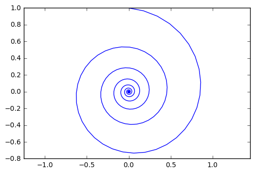
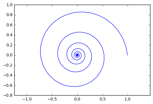
I want output and inline figures. This ipython block should output some text and two figures. Note we do not define file names anywhere! See this section for details on how to get ob-ipython to do this.

%matplotlib inline
import matplotlib.pyplot as plt
import numpy as np

t = np.linspace(0, 20 * np.pi, 350)
x = np.exp(-0.1 * t) * np.sin(t)
y = np.exp(-0.1 * t) * np.cos(t)

plt.plot(x, y)
plt.axis('equal')

plt.figure()
plt.plot(y, x)
plt.axis('equal')

print('Length of t = {}'.format(len(t)))
print('x .dot. y = {}'.format(x @ y))

Length of t = 350 x .dot. y = 1.3598389888491538

Nice, success! Now my code blocks export more cleanly to jupyter notebooks. Speaking of which, if you liked the post on that, there is a new library for it in scimax: https://github.com/jkitchin/scimax/blob/master/ox-ipynb.el. Yes, one day I will put it in its own repo, and probably put it up on MELPA. If it turns out to be useful over the next semester.

1 code for getting output and inline figures

I wrote one new function that writes the base64 data out to a temporary file and returns a link to it. Then, I modified the org-babel-execute:ipython function to append these links onto the output. It seems like you need to use a header like this in your ob-ipython block, notably the results need to be in a drawer like this if you want org-mode to render the images. They do not show up in the results that have colons starting them.

#+BEGIN_SRC ipython :session :results output drawer

Here is the code.

(defun ob-ipython-inline-image (b64-string)
  "Write the b64-string to a temporary file.
Returns an org-link to the file."
  (let* ((tfile (make-temp-file "ob-ipython-" nil ".png"))
         (link (format "[[file:%s]]" tfile)))
    (ob-ipython--write-base64-string tfile b64-string)
    link))


(defun org-babel-execute:ipython (body params)
  "Execute a block of IPython code with Babel.
This function is called by `org-babel-execute-src-block'."
  (let* ((file (cdr (assoc :file params)))
         (session (cdr (assoc :session params)))
         (result-type (cdr (assoc :result-type params))))
    (org-babel-ipython-initiate-session session params)
    (-when-let (ret (ob-ipython--eval
                     (ob-ipython--execute-request
                      (org-babel-expand-body:generic (encode-coding-string body 'utf-8)
                                                     params (org-babel-variable-assignments:python params))
                      (ob-ipython--normalize-session session))))
      (let ((result (cdr (assoc :result ret)))
            (output (cdr (assoc :output ret))))
        (if (eq result-type 'output)
            (concat
             output 
             (format "%s"
                     (mapconcat 'identity
                                (loop for res in result
                                      if (eq 'image/png (car res))
                                      collect (ob-ipython-inline-image (cdr res)))
                                "\n")))
          (ob-ipython--create-stdout-buffer output)
          (cond ((and file (string= (f-ext file) "png"))
                 (->> result (assoc 'image/png) cdr (ob-ipython--write-base64-string file)))
                ((and file (string= (f-ext file) "svg"))
                 (->> result (assoc 'image/svg+xml) cdr (ob-ipython--write-string-to-file file)))
                (file (error "%s is currently an unsupported file extension." (f-ext file)))
                (t (->> result (assoc 'text/plain) cdr))))))))
org-babel-execute:ipython

Copyright (C) 2017 by John Kitchin. See the License for information about copying.

org-mode source

Org-mode version = 9.0.3

Discuss on Twitter

Exporting org-mode to Jupyter notebooks

| categories: python, jupyter, orgmode, emacs | tags:

I am going to use Jupyter notebooks to teach from this semester. I really dislike preparing notebooks though. A browser is a really poor editor, and I really dislike Markdown. Notebooks do not seem to have any real structure in them, e.g. the collapsible outline that I am used to in org-mode, so for long notebooks, it is difficult to get a sense for the structure. I am anticipating spending up to 80 hours preparing notebooks this semester, so today I worked out some code to export org-mode to an ipython notebook!

This will let me use the power tools I am accustomed to for the creation of IPython notebooks for my students, and perhaps others who do not use org-mode.

Jupyter notebooks are just json files, so all we need to do is generate it from an org document. The basic strategy was to build up a lisp data structure that represents the notebook and then just convert that data structure to json. I split the document up into sequential markdown and code cells, and then encode those in the format required for the notebook (json).

So, here is an example of what can be easily written in org-mode, posted to this blog, and exported to an IPython notebook, all from one org-document.

Check out the notebook: exporting-orgmode-to-ipynb.ipynb .

1 Solve a nonlinear problem

Consider the equation \(x^2 = 4\). Find a solution to it in Python using a nonlinear solver.

To do that, we need to define an objective function that will be equal to zero at the solution. Here is the function:

def objective(x):
    return x**2 - 4

Next, we use fsolve with an initial guess. We get fsolve from scipy.optimize.

from scipy.optimize import fsolve

ans = fsolve(objective, 3)
print(ans)
[ 2.]

That should have been an obvious answer. The answer is in brackets because fsolve returns an array. In the next block we will unpack the solution into the answer using the comma operator. Also, we can see that using a different guess leads to a different answer. There are, of course, two answers: \(x = \pm 2\)

ans, = fsolve(objective, -3)
print(ans)
-2.0

Now you see we get a float answer!

Here are some other ways to get a float:

ans = fsolve(objective, -3)

print(float(ans))
print(ans[0])
-2.0000000000000084
-2.0

It is worth noting from the first result that fsolve is iterative and stops when it reaches zero within a tolerance. That is why it is not exactly -2.

2 Benefits of export to ipynb

  1. I can use org-mode
  2. And emacs
  3. and ipynb for teaching.

The export supports org-markup: bold, italic, underlined, and ~~strike~~.

We can use tables:

Table 1: A table of squares.
x y
1 2
2 4
3 9
4 16

We can make plots.

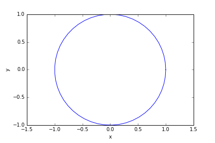
import numpy as np

t = np.linspace(0, 2 * np.pi)

x = np.cos(t)
y = np.sin(t)

import matplotlib.pyplot as plt
plt.plot(x, y)
plt.axis('equal')
plt.xlabel('x')
plt.ylabel('y')
plt.savefig('circle.png')

Even include HTML: <font color="red">Pay special attention to the axis labels!</font>

3 Limitations

  • Only supports iPython blocks
  • Does not do inline images in results
  • Will not support src-block variables
  • Currently only supports vanilla output results

4 Summary

The code that does this is here: ox-ipynb.el . After I use it a while I will put it in scimax. There are some tricks in it to fix up some markdown export of latex fragments and links with no descriptions.

I just run this command in Emacs to get the notebook. Even it renders reasonably in the notebook.

(export-ipynb-buffer)

Overall, this looks extremely promising to develop lecture notes and assignments in org-mode, but export them to Ipython notebooks for the students.

Copyright (C) 2017 by John Kitchin. See the License for information about copying.

org-mode source

Org-mode version = 9.0.3

Discuss on Twitter

Querying a MongoDB bibtex database with Python and emacs-lisp

| categories: database, python, mongodb, emacs | tags:

I have been exploring using databases to help with searching my data. In this post we explore using MongoDB for bibtex entries. I am choosing bibtex entries because it is easy to parse bibtex files, I already have a lot of them, and I have several kinds of queries I regularly use. So, they are a good candidate to test out a new database on!

MongoDB is a noSQL database that is pretty easy to use. I installed it from homebrew, and then followed the directions to run the server.

With pymongo you can make a database as easy as this:

import bibtexparser

# Read the bibtex file to get entries
with open('../../../Dropbox/bibliography/references.bib', 'r') as bibfile:
    bp = bibtexparser.load(bibfile)
    entries = bp.entries

print("N = ", len(entries))

print(entries[0])

import pymongo
from pymongo import MongoClient
client = MongoClient('localhost', 27017)

# This creates the "entries" collection
db = client['bibtex'].entries

# add each entry
for entry in entries:
    db.insert_one(entry)

N = 1671 {'keyword': 'test, word', 'year': '2006', 'publisher': 'American Chemical Society (ACS)', 'title': 'The ACS Style Guide', 'ENTRYTYPE': 'book', 'editor': 'Janet S. Dodd', 'address': 'Washington, D.C.', 'ID': '2006-acs-style-guide', 'doi': '10.1021/bk-2006-styg', 'link': 'https://doi.org/10.1021/bk-2006-STYG', 'date_added': 'Wed Apr 1 10:17:54 2015', 'pages': 'nil'}

That was easy. We have a database with 1671 documents in it, and each document is essentially a dictionary of key-value pairs. You might even argue it was too easy. I didn't specify any structure to the entries at all. No required fields, no validation that the keys are spelled correctly, no validation on the values, e.g. you can see the year looks like a string. The benefit of that is that every entry went in, with no issues. On the other hand, the authors went in as a single string, as did the keywords, which affects our ability to search a little bit later. Note if you run that twice, it will add each entry again, since we do not check if the entry already exists.

A database is only useful though if it is easy to get stuff out of it. So, let's consider some test queries. First we find entries that have years less than 1950. The query is basically a little json bundle that describes a field and condition that we want to match. Here we use a less than operator, ""$lt"The results come back as a list of dictionaries. This is in stark contrast to a SQL query which is an expression in its own declarative language. A query here is a chunk of data that must get converted to code by the server. I am not 100% clear if the less than here is in the string sense or numeric sense, but for years it probably does not matter for a long time.

import pymongo
from pymongo import MongoClient
client = MongoClient('localhost', 27017)

db = client['bibtex'].entries

for i, result in enumerate(db.find({"year" : {"$lt": "1950"}})):
    print('{i: 2d}. {author}, {title}, {journal}, {year}.'.format(i=i+1, **result))
  1. Birch, Francis, Finite Elastic Strain of Cubic Crystals, Phys. Rev., 1947.
  2. Ditchburn, R. W. and Gilmour, J. C., The Vapor Pressures of Monatomic Vapors, Rev. Mod. Phys., 1941.
  3. J. Korringa, On the Calculation of the Energy of a Bloch Wave in a Metal, Physica, 1947.
  4. Nix, F. C. and MacNair, D., The Thermal Expansion of Pure Metals. {II}: Molybdenum, Palladium, Silver, Tantalum, Tungsten, Platinum, and Lead, Phys. Rev., 1942.

That seems easy enough, and those strings could easily be used as candidates for a selection tool like helm.

How about articles published by myself and my student Jacob Boes? This requires "and" logic. Apparently that is the default, so we just add three queries. One is an exact match on articles, and the other two are case-insensitive regular expression matches. I guess this has to be done on every document, since there probably is no way to index a regex match! This search was very fast, but it is not clear how fast it would be for a million entries. This matching is necessary because we stored all authors in a single field rather than splitting them into an array. We might still have to match strings for this even in an array since an author might then be "John R. Kitchin", rather than further decomposed into first and last names.

import pymongo
from pymongo import MongoClient
client = MongoClient('localhost', 27017)

db = client['bibtex']
entries = db['entries']

for i, result in enumerate(entries.find({"ENTRYTYPE": "article",
                                         "author" : {"$regex": "kitchin", '$options' : 'i'},
                                         "author" : {"$regex": "boes", '$options' : 'i'}})):
    if result.get('doi', None):
        result['doi'] = 'https://doi.org/{doi}'.format(doi=result['doi'])
    else:
        result['doi'] = ''
    print('{i: 2d}. {author}, {title}, {journal}, {year}. {doi}'.format(i=i+1, **result).replace("\n", ""))
  1. Jacob R. Boes and Peter Kondratyuk and Chunrong Yin and JamesB. Miller and Andrew J. Gellman and John R. Kitchin, Core Level Shifts in {Cu-Pd} Alloys As a Function of BulkComposition and Structure, Surface Science, 2015. https://doi.org/10.1016/j.susc.2015.02.011
  2. Jacob R. Boes and Gamze Gumuslu and James B. Miller and AndrewJ. Gellman and John R. Kitchin, Estimating Bulk-Composition-Dependent \ce{H2} AdsorptionEnergies on \ce{CuxPd1-x} Alloy (111) Surfaces, ACS Catalysis, 2015. https://doi.org/10.1021/cs501585k
  3. Jacob R. Boes and Gamze Gumuslu and James B. Miller and AndrewJ. Gellman and John R. Kitchin, Supporting Information: Estimating Bulk-Composition-Dependent\ce{H2} Adsorption Energies on \ce{CuxPd1-x} Alloy (111)Surfaces, ACS Catalysis, 2015. https://doi.org/10.1021/cs501585k
  4. G. Gumuslu and P. Kondratyuk and J. R. Boes and B. Morrealeand J. B. Miller and J. R. Kitchin and A. J. Gellman, Correlation of Electronic Structure With Catalytic Activity:\ce{H2}-\ce{D2} Exchange Across \ce{CuxPd1-x}Composition Space, ACS Catalysis, 2015. https://doi.org/10.1021/cs501586t
  5. John D. Michael and Ethan L. Demeter and Steven M. Illes andQingqi Fan and Jacob R. Boes and John R. Kitchin, Alkaline Electrolyte and {Fe} Impurity Effects on thePerformance and Active-Phase Structure of {NiOOH} Thin Filmsfor {OER} Catalysis Applications, J. Phys. Chem. C, 2015. https://doi.org/10.1021/acs.jpcc.5b02458
  6. Jacob R. Boes and Mitchell C. Groenenboom and John A. Keithand John R. Kitchin, Neural Network and {Reaxff} Comparison for {Au} Properties, Int. J. Quantum Chem., 2016. https://doi.org/10.1002/qua.25115
  7. Jacob R. Boes and John R. Kitchin, Neural Network Predictions of Oxygen Interactions on a Dynamic Pd Surface, Molecular Simulation, Accepted 12/2016. https://doi.org/10.1080/08927022.2016.1274984
  8. Jacob R. Boes and John R. Kitchin, Modeling Segregation on {AuPd}(111) Surfaces With DensityFunctional Theory and Monte Carlo Simulations, Submitted to J. Phys. Chem. C, 2016.

We can find out how many different entry types we have, as well as how many distinct keyword entries there are. The documents do not separate the keywords though, so this is just the unique strings of comma-separated keywords values. We would have had to split those in advance to have a list of keywords to search for a specific one beyond string matching. Curiously, in my bibtex entries, these are in a field called "keywords". It appears the bibtex parser may have changed the name to "keyword".

import pymongo
from pymongo import MongoClient
client = MongoClient('localhost', 27017)

db = client['bibtex']
entries = db['entries']

print(entries.distinct("ENTRYTYPE"))
print(len(entries.distinct("keyword")))
print(entries.find({"keyword": {"$exists": "true"}})[22]['keyword'])

['book', 'article', 'techreport', 'phdthesis', 'inproceedings', 'inbook', 'mastersthesis', 'misc', 'incollection'] 176 Bildungsw{\"a}rmen, Dichtefunktionalrechnungen, Perowskite, Thermochemie

1 text searching

You can do text search as well. You first have to create an index on one or more fields, and then use the $text and $search operators. Here I made an index on a few fields, and then searched on it. Note that you can only have one text index, so think about it in advance! This simplifies the query a bit, we do not have to use the regex syntax for matching on a field.

import pymongo
from pymongo import MongoClient
client = MongoClient('localhost', 27017)

db = client['bibtex']
entries = db['entries']

entries.create_index([('author', pymongo.TEXT),
                      ('title', pymongo.TEXT),
                      ('keyword', pymongo.TEXT)], sparse=True)

for i, result in enumerate(entries.find({"$text" : {"$search": "kitchin", "$search": "boes"}})):
    print('{i: 2d}. {author}, {title}, {journal}, {year}.'.format(i=i, **result).replace("\n", ""))
  1. G. Gumuslu and P. Kondratyuk and J. R. Boes and B. Morrealeand J. B. Miller and J. R. Kitchin and A. J. Gellman, Correlation of Electronic Structure With Catalytic Activity:\ce{H2}-\ce{D2} Exchange Across \ce{CuxPd1-x}Composition Space, ACS Catalysis, 2015.
  2. Jacob R. Boes and Peter Kondratyuk and Chunrong Yin and JamesB. Miller and Andrew J. Gellman and John R. Kitchin, Core Level Shifts in {Cu-Pd} Alloys As a Function of BulkComposition and Structure, Surface Science, 2015.
  3. Jacob R. Boes and Gamze Gumuslu and James B. Miller and AndrewJ. Gellman and John R. Kitchin, Estimating Bulk-Composition-Dependent \ce{H2} AdsorptionEnergies on \ce{CuxPd1-x} Alloy (111) Surfaces, ACS Catalysis, 2015.
  4. Jacob R. Boes and John R. Kitchin, Neural Network Predictions of Oxygen Interactions on a Dynamic Pd Surface, Molecular Simulation, Accepted 12/2016.
  5. Jacob R. Boes and John R. Kitchin, Modeling Segregation on {AuPd}(111) Surfaces With DensityFunctional Theory and Monte Carlo Simulations, Submitted to J. Phys. Chem. C, 2016.
  6. Jacob R. Boes and Gamze Gumuslu and James B. Miller and AndrewJ. Gellman and John R. Kitchin, Supporting Information: Estimating Bulk-Composition-Dependent\ce{H2} Adsorption Energies on \ce{CuxPd1-x} Alloy (111)Surfaces, ACS Catalysis, 2015.
  7. John D. Michael and Ethan L. Demeter and Steven M. Illes andQingqi Fan and Jacob R. Boes and John R. Kitchin, Alkaline Electrolyte and {Fe} Impurity Effects on thePerformance and Active-Phase Structure of {NiOOH} Thin Filmsfor {OER} Catalysis Applications, J. Phys. Chem. C, 2015.
  8. Jacob R. Boes and Mitchell C. Groenenboom and John A. Keithand John R. Kitchin, Neural Network and {Reaxff} Comparison for {Au} Properties, Int. J. Quantum Chem., 2016.

We can use this to search for documents with orgmode in a keyword or title too.

import pymongo
from pymongo import MongoClient
client = MongoClient('localhost', 27017)

db = client['bibtex']
entries = db['entries']

entries.create_index([('author', pymongo.TEXT),
                      ('title', pymongo.TEXT),
                      ('keyword', pymongo.TEXT)], sparse=True)

for i, result in enumerate(entries.find({"$text" : {"$search": "orgmode"}})):
    print('{i: 2d}. {author}, {title}, {journal}, {year}.'.format(i=i, **result).replace("\n", ""))
  1. John R. Kitchin, Data Sharing in Surface Science, Surface Science, 2016.
  2. Zhongnan Xu and John R. Kitchin, Probing the Coverage Dependence of Site and AdsorbateConfigurational Correlations on (111) Surfaces of LateTransition Metals, J. Phys. Chem. C, 2014.
  3. Xu, Zhongnan and Rossmeisl, Jan and Kitchin, John R., A Linear Response {DFT}+{U} Study of Trends in the OxygenEvolution Activity of Transition Metal Rutile Dioxides, The Journal of Physical Chemistry C, 2015.
  4. Prateek Mehta and Paul A. Salvador and John R. Kitchin, Identifying Potential \ce{BO2} Oxide Polymorphs for EpitaxialGrowth Candidates, ACS Appl. Mater. Interfaces, 2015.
  5. Xu, Zhongnan and Joshi, Yogesh V. and Raman, Sumathy andKitchin, John R., Accurate Electronic and Chemical Properties of 3d TransitionMetal Oxides Using a Calculated Linear Response {U} and a {DFT+ U(V)} Method, The Journal of Chemical Physics, 2015.
  6. Zhongnan Xu and John R. Kitchin, Relationships Between the Surface Electronic and ChemicalProperties of Doped 4d and 5d Late Transition Metal Dioxides, The Journal of Chemical Physics, 2015.
  7. Zhongnan Xu and John R Kitchin, Tuning Oxide Activity Through Modification of the Crystal andElectronic Structure: From Strain To Potential Polymorphs, Phys. Chem. Chem. Phys., 2015.
  8. Jacob R. Boes and Gamze Gumuslu and James B. Miller and AndrewJ. Gellman and John R. Kitchin, Supporting Information: Estimating Bulk-Composition-Dependent\ce{H2} Adsorption Energies on \ce{CuxPd1-x} Alloy (111)Surfaces, ACS Catalysis, 2015.
  9. Kitchin, John R., Examples of Effective Data Sharing in Scientific Publishing, ACS Catalysis, 2015.
  10. Curnan, Matthew T. and Kitchin, John R., Effects of Concentration, Crystal Structure, Magnetism, andElectronic Structure Method on First-Principles Oxygen VacancyFormation Energy Trends in Perovskites, The Journal of Physical Chemistry C, 2014.
  11. Kitchin, John R. and Van Gulick, Ana E. and Zilinski, Lisa D., Automating Data Sharing Through Authoring Tools, International Journal on Digital Libraries, 2016.
  12. Jacob R. Boes and Gamze Gumuslu and James B. Miller and AndrewJ. Gellman and John R. Kitchin, Estimating Bulk-Composition-Dependent \ce{H2} AdsorptionEnergies on \ce{CuxPd1-x} Alloy (111) Surfaces, ACS Catalysis, 2015.
  13. Zhongnan Xu and John R. Kitchin, Relating the Electronic Structure and Reactivity of the 3dTransition Metal Monoxide Surfaces, Catalysis Communications, 2014.
  14. Spencer D. Miller and Vladimir V. Pushkarev and AndrewJ. Gellman and John R. Kitchin, Simulating Temperature Programmed Desorption of Oxygen on{P}t(111) Using {DFT} Derived Coverage Dependent DesorptionBarriers, Topics in Catalysis, 2014.
  15. Hallenbeck, Alexander P. and Kitchin, John R., Effects of \ce{O_2} and \ce{SO_2} on the Capture Capacity of aPrimary-Amine Based Polymeric \ce{CO_2} Sorbent, Industrial \& Engineering Chemistry Research, 2013.

2 Querying from emacs-lisp

It is hard to get too excited about this if it is not easy to query from emacs and get data in a form we can use in emacs ;) The json library allows us to convert lisp data structures to json pretty easily. For example:

(require 'json)

(json-encode '((ENTRYTYPE . article)
               (author . (($regex . kitchin)
                          ($options . i)))
               (author . (($regex . boes)
                          ($options . i)))))
{"ENTRYTYPE":"article","author":{"$regex":"kitchin","$options":"i"},"author":{"$regex":"boes","$options":"i"}}

So, we can use an a-list syntax to build up the query. Then we can send it to mongo using mongoexport that will return a json string that we can read back into emacs to get lisp data. Here is an example that returns a query. We print the first element here.

(pp
 (aref (json-read-from-string
        (shell-command-to-string
         (format "mongoexport --quiet --jsonArray -d bibtex -c entries -q '%s'"
                 (json-encode '((ENTRYTYPE . article)
                                (author . (($regex . kitchin)
                                           ($options . i)))
                                (author . (($regex . boes)
                                           ($options . i))))))))
       0))
((_id
  ($oid . "5878d9644c114f59fe86cb36"))
 (author . "Jacob R. Boes and Peter Kondratyuk and Chunrong Yin and James\nB. Miller and Andrew J. Gellman and John R. Kitchin")
 (year . "2015")
 (title . "Core Level Shifts in {Cu-Pd} Alloys As a Function of Bulk\nComposition and Structure")
 (ENTRYTYPE . "article")
 (ID . "boes-2015-core-cu")
 (keyword . "DESC0004031, early-career")
 (volume . "640")
 (doi . "10.1016/j.susc.2015.02.011")
 (link . "https://doi.org/10.1016/j.susc.2015.02.011")
 (issn . "0039-6028")
 (journal . "Surface Science")
 (pages . "127-132"))

That is pretty sweet, we get a lisp data structure we can use. We can wrap that into a reasonable looking function here:

(defun mongo-find (db collection query)
  (json-read-from-string
   (shell-command-to-string
    (format "mongoexport --quiet --jsonArray -d %s -c %s -q '%s'"
            db collection (json-encode query)))))
mongo-find

Now we can use the function to query the database, and then format the results. Here we look at the example of articles with authors that match "kitchin" and "boes".

(loop for counter from 1 for entry across
      (mongo-find "bibtex" "entries" '((ENTRYTYPE . article)
                                       (author . (($regex . kitchin)
                                                  ($options . i)))
                                       (author . (($regex . boes)
                                                  ($options . i)))))
      do
      (setq entry (append `(,(cons "counter" counter)) entry))
      ;; make sure we have a doi field.
      (if (assoc 'doi entry)
          (push (cons "doi" (format "https://doi.org/%s" (cdr (assoc 'doi entry)))) entry)
        (push (cons "doi" "") entry))
      concat
      (concat (replace-regexp-in-string
               "\n" " "
               (s-format "${counter}. ${author}, ${title} (${year}). ${doi}"
                         'aget entry)) "\n"))
1. Jacob R. Boes and Peter Kondratyuk and Chunrong Yin and James B. Miller and Andrew J. Gellman and John R. Kitchin, Core Level Shifts in {Cu-Pd} Alloys As a Function of Bulk Composition and Structure (2015). https://doi.org/10.1016/j.susc.2015.02.011
2. Jacob R. Boes and Gamze Gumuslu and James B. Miller and Andrew J. Gellman and John R. Kitchin, Estimating Bulk-Composition-Dependent \ce{H2} Adsorption Energies on \ce{Cu_{x}Pd_{1-x}} Alloy (111) Surfaces (2015). https://doi.org/10.1021/cs501585k
3. Jacob R. Boes and Gamze Gumuslu and James B. Miller and Andrew J. Gellman and John R. Kitchin, Supporting Information: Estimating Bulk-Composition-Dependent \ce{H2} Adsorption Energies on \ce{Cu_{x}Pd_{1-x}} Alloy (111) Surfaces (2015). https://doi.org/10.1021/cs501585k
4. G. Gumuslu and P. Kondratyuk and J. R. Boes and B. Morreale and J. B. Miller and J. R. Kitchin and A. J. Gellman, Correlation of Electronic Structure With Catalytic Activity: \ce{H2}-\ce{D2} Exchange Across \ce{Cu_{x}Pd_{1-x}} Composition Space (2015). https://doi.org/10.1021/cs501586t
5. John D. Michael and Ethan L. Demeter and Steven M. Illes and Qingqi Fan and Jacob R. Boes and John R. Kitchin, Alkaline Electrolyte and {Fe} Impurity Effects on the Performance and Active-Phase Structure of {NiOOH} Thin Films for {OER} Catalysis Applications (2015). https://doi.org/10.1021/acs.jpcc.5b02458
6. Jacob R. Boes and Mitchell C. Groenenboom and John A. Keith and John R. Kitchin, Neural Network and {Reaxff} Comparison for {Au} Properties (2016). https://doi.org/10.1002/qua.25115
7. Jacob R. Boes and John R. Kitchin, Neural Network Predictions of Oxygen Interactions on a Dynamic Pd Surface (Accepted 12/2016). https://doi.org/10.1080/08927022.2016.1274984
8. Jacob R. Boes and John R. Kitchin, Modeling Segregation on {AuPd}(111) Surfaces With Density Functional Theory and Monte Carlo Simulations (2016).

Wow, that looks like a pretty lispy way to query the database and use the results. It is probably pretty easy to do similar things for inserting and updating documents. I will save that for another day.

3 Summary thoughts

This is not an exhaustive study of Mongo for a bibtex database. It does illustrate that it is potentially useful. Imagine a group of users can enter bibtex entries, and then share them through a central server. Or you query the server for entries and then select them using helm/ivy. That is probably faster than parsing large bibtex files (note, in org-ref I already cache the files in parsed form for performance reasons!).

It would make sense to split the authors, and keywords in another version of this database. It also could make sense to have a field that is the bibtex string, and to do text search on that string. That way you get everything in the entry for searching, and an easy way to generate bibtex files without having to reconstruct them.

It is especially interesting to run the queries through emacs-lisp since we get the benefit of editing lisp code while writing the query, e.g. parenthesis navigation, less quoting, etc… and we get back lisp data that can be used to construct helm/ivy queries, or other emacs things. That makes this look competitive with emacsql at least for the syntax. I predict that there will be more posts on this in the future.

Copyright (C) 2017 by John Kitchin. See the License for information about copying.

org-mode source

Org-mode version = 9.0.3

Discuss on Twitter

New and improved asynchronous org-babel python blocks

| categories: python, orgmode, emacs | tags:

Table of Contents

About a year ago I posted some code to run org-babel python blocks asynchronously. This year, my students asked for some enhancements related to debugging. Basically, they were frustrated by a few things when they got errors. First, they found it difficult to find the line number in the Traceback in the src block because there are no line numbers in the block, and it is annoying to do a special edit just for line numbers.

I thought about this, and figured out how to significantly improve the situation. The async python code in scimax now has the following features:

  1. When you get a Traceback, it goes in the results, and each file listed in it is hyperlinked to the source file and line so it is easy to get to them.
  2. The cursor jumps to the last line in the code block that is listed in the Traceback, and a beacon shines to show you the line
  3. You can turn on temporary line numbers in the code block to see where the lines are in the block, and these disappear when you start typing. This is done in the variable `org-babel-async-python-show-line-numbers'.
  4. You can control whether a buffer of the results shows or not via the variable `org-babel-async-python-show-results'.
  5. When you run the block, you get a clickable link in the RESULTS section to kill the process.
  6. You may also find the `autopep8' and `pylint' functions helpful.

The code for this is currently found here: https://github.com/jkitchin/scimax/blob/org-9/scimax-org-babel-python.el

Eventually, I will merge this into master, after I am sure about all the changes needed for org 9.0. That is not likely to happen until the semester ends, so I do not mess up my students who use scimax in class. So, sometime mid-December it will make into master.

To make async the default way to run a python block use this code, so that you can use C-c C-c to run them:

(require 'scimax-org-babel-python)
(add-to-list 'org-ctrl-c-ctrl-c-hook 'org-babel-async-execute:python)

As with the past few posts, this video will make it much more clear what the post is about:

Here is a prototypical example that shows how it works. While it runs you can view the progress if you click on the link to show the results.

import time

for i in range(5):
    print(i)
    time.sleep(2)

0 1 2 3 4 Traceback (most recent call last): File "Org SRC", line 5, in <module> time.sleep(2) KeyboardInterrupt

This block has a pretty obvious issue when we run it. The cursor jumps right to the problem!

print('This line is ok')
# 5 / 0
print('We will not see this')

This line is ok We will not see this

This block shows we can access any of the links in the Traceback. Here we have an error in calling a function that is raised in an external file.

import numpy as np
from scipy.integrate import odeint

Vspan = np.linspace(0, 2) # L

# dF/dV = F
def dFdV(F, V, v0):
    return F


print(odeint(dFdV, 1.0, Vspan))

Traceback (most recent call last): File "Org SRC", line 11, in <module> print(odeint(dFdV, 1.0, Vspan)) File "/Users/jkitchin/anaconda3/lib/python3.5/site-packages/scipy/integrate/odepack.py", line 215, in odeint ixpr, mxstep, mxhnil, mxordn, mxords) TypeError: dFdV() missing 1 required positional argument: 'v0'

Here we show how nice it is to be able to kill a process. This block will not end on its own.

while True:
    pass

Traceback (most recent call last): File "Org SRC", line 2, in <module> pass KeyboardInterrupt

1 autopep8

autopep8 is a tool for reformatting Python code. We wrapped this into an Emacs command so you can quickly reformat a Python code block.

a = 4
b = 5
c = a * b  # comment
# another comment


def f(x):
    return x
print(f(5))

2 pylint

pylint is a great tool for checking your Python code for errors, style and conventions. We also wrapped this into an Emacs command so you can run it on a Python src block. The report that is generated had clickable links to help you get right to the lines in your code block with problems.

import numpy as np

a = np.array(5, 5)

def f(x): return x

print(f(6))

Copyright (C) 2016 by John Kitchin. See the License for information about copying.

org-mode source

Org-mode version = 9.0

Discuss on Twitter
« Previous Page -- Next Page »