Modeling a Cu dimer by EMT, nonlinear regression and neural networks
Posted March 18, 2017 at 03:47 PM | categories: machine-learning, molecular-simulation, neural-network, python | tags:
In this post we consider a Cu2 dimer and how its energy varies with the separation of the atoms. We assume we have a way to calculate this, but that it is expensive, and that we want to create a simpler model that is as accurate, but cheaper to run. A simple way to do that is to regress a physical model, but we will illustrate some challenges with that. We then show a neural network can be used as an accurate regression function without needing to know more about the physics.
We will use an effective medium theory calculator to demonstrate this. The calculations are not expected to be very accurate or relevant to any experimental data, but they are fast, and will illustrate several useful points that are independent of that. We will take as our energy zero the energy of two atoms at a large separation, in this case about 10 angstroms. Here we plot the energy as a function of the distance between the two atoms, which is the only degree of freedom that matters in this example.
import numpy as np
%matplotlib inline
import matplotlib.pyplot as plt

from ase.calculators.emt import EMT
from ase import Atoms

atoms = Atoms('Cu2',[[0, 0, 0], [10, 0, 0]], pbc=[False, False, False])
atoms.set_calculator(EMT())

e0 = atoms.get_potential_energy()

# Array of bond lengths to get the energy for
d = np.linspace(1.7, 3, 30)

def get_e(distance):
    a = atoms.copy()
    a[1].x = distance
    a.set_calculator(EMT())
    e = a.get_potential_energy()
    return e

e = np.array([get_e(dist) for dist in d])
e -=  e0  # set the energy zero

plt.plot(d, e, 'bo ')
plt.xlabel('d (Å)')
plt.ylabel('energy (eV)')
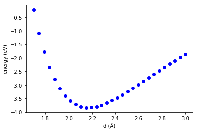
We see there is a minimum, and the energy is asymmetric about the minimum. We have no functional form for the energy here, just the data in the plot. So to get another energy, we have to run another calculation. If that was expensive, we might prefer an analytical equation to evaluate instead. We will get an analytical form by fitting a function to the data. A classic one is the Buckingham potential: \(E = A \exp(-B r) - \frac{C}{r^6}\). Here we perform the regression.
def model(r, A, B, C):
    return A * np.exp(-B * r) - C / r**6

from pycse import nlinfit
import pprint

p0 = [-80, 1, 1]
p, pint, se = nlinfit(model, d, e, p0, 0.05)
print('Parameters = ', p)
print('Confidence intervals = ')
pprint.pprint(pint)
plt.plot(d, e, 'bo ', label='calculations')

x = np.linspace(min(d), max(d))
plt.plot(x, model(x, *p), label='fit')
plt.legend(loc='best')
plt.xlabel('d (Å)')
plt.ylabel('energy (eV)')
Parameters = [ -83.21072545 1.18663393 -266.15259507]
Confidence intervals =
array([[ -93.47624687, -72.94520404],
[ 1.14158438, 1.23168348],
[-280.92915682, -251.37603331]])
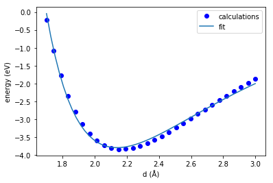
That fit is ok, but not great. We would be better off with a spline for this simple system! The trouble is how do we get anything better? If we had a better equation to fit to we might get better results. While one might come up with one for this dimer, how would you extend it to more complex systems, even just a trimer? There have been decades of research dedicated to that, and we are not smarter than those researchers so, it is time for a new approach.
We will use a Neural Network regressor. The input will be \(d\) and we want to regress a function to predict the energy.
There are a couple of important points to make here.
- This is just another kind of regression.
- We need a lot more data to do the regression. Here we use 300 data points.
- We need to specify a network architecture. Here we use one hidden layer with 10 neurons, and the tanh activation function on each neuron. The last layer is just the output layer. I do not claim this is any kind of optimal architecture. It is just one that works to illustrate the idea.
Here is the code that uses a neural network regressor, which is lightly adapted from http://scikit-neuralnetwork.readthedocs.io/en/latest/guide_model.html.
from sknn.mlp import Regressor, Layer

D = np.linspace(1.7, 3, 300)

def get_e(distance):
    a = atoms.copy()
    a[1].x = distance
    a.set_calculator(EMT())
    e = a.get_potential_energy()
    return e

E = np.array([get_e(dist) for dist in D])
E -=  e0  # set the energy zero

X_train = np.row_stack(np.array(D))

N = 10
nn = Regressor(layers=[Layer("Tanh", units=N),
                       Layer('Linear')])
nn.fit(X_train, E)

dfit = np.linspace(min(d), max(d))

efit = nn.predict(np.row_stack(dfit))

plt.plot(d, e, 'bo ')
plt.plot(dfit, efit)
plt.legend(['calculations', 'neural network'])
plt.xlabel('d (Å)')
plt.ylabel('energy (eV)')
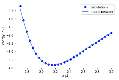
This fit looks pretty good, better than we got for the Buckingham potential. Well, it probably should look better, we have many more parameters that were fitted! It is not perfect, but it could be systematically improved by increasing the number of hidden layers, and neurons in each layer. I am being a little loose here by relying on a visual assessment of the fit. To systematically improve it you would need a quantitative analysis of the errors. I also note though, that if I run the block above several times in succession, I get different fits each time. I suppose that is due to some random numbers used to initialize the fit, but sometimes the fit is about as good as the result you see above, and sometimes it is terrible.
Ok, what is the point after all? We developed a neural network that pretty accurately captures the energy of a Cu dimer with no knowledge of the physics involved. Now, EMT is not that expensive, but suppose this required 300 DFT calculations at 1 minute or more a piece? That is five hours just to get the data! With this neural network, we can quickly compute energies. For example, this shows we get about 10000 energy calculations in just 287 ms.
%%timeit

dfit = np.linspace(min(d), max(d), 10000)
efit = nn.predict(np.row_stack(dfit))
1 loop, best of 3: 287 ms per loop
Compare that to the time it took to compute the 300 energies with EMT
%%timeit
E = np.array([get_e(dist) for dist in D])
1 loop, best of 3: 230 ms per loop
The neural network is a lot faster than the way we get the EMT energies!
It is true in this case we could have used a spline, or interpolating function and it would likely be even better than this Neural Network. We are aiming to get more complicated soon though. For a trimer, we will have three dimensions to worry about, and that can still be worked out in a similar fashion I think. Past that, it becomes too hard to reduce the dimensions, and this approach breaks down. Then we have to try something else. We will get to that in another post.
Copyright (C) 2017 by John Kitchin. See the License for information about copying.
Org-mode version = 9.0.5