Lies, damn lies, statistics and Bayesian statistics
Posted June 22, 2025 at 11:14 AM | categories: machine-learning | tags:
Updated June 23, 2025 at 01:33 PM
Table of Contents
This post on LinkedIn (https://www.linkedin.com/posts/activity-7341134401705041920-gaEd?utm_source=share&utm_medium=member_desktop&rcm=ACoAAAfqmO0BzyXpJw8w7yyHwkoMSiaKfGg-sKI) reminded me of a quip I often make of "Lies, damn lies, statistics, and Bayesian statistics". I am frequently skeptical of claims about "Bayesian something something", especially when the claim is about uncertainty quantification. That skepticism comes from practical experience of mine that "Bayesian something something" is rarely as well behaved and informative as advertised (in my hands of course).
To illustrate, I will use some noisy, 1d data from a Lennard-Jones function and Gaussian process regression to fit the data.
1. The data
We get our data by sampling a Lennard-Jones function, adding some noise, and removing a gap in the data. The gap in the middle might be classically considered an interpolation region.
import numpy as np
import matplotlib.pyplot as plt

r = np.linspace(0.95, 3, 200)

eps, sig = 1, 1
y = 4 * eps * ((1 / r)**12 - (1 / r)**6) + np.random.normal(0, 0.03, size=r.shape)


ind = ((r > 1) & (r < 1.25)) | ((r > 2) & (r < 2.5))
_R = r[ind][:, None]
_y = y[ind]
plt.plot(_R, _y, '.')
plt.xlabel('R')
plt.ylabel('E');

2. GPR with a RBF kernel
The RBF kernel is the most standard kernel. It does an ok job fitting here, although I see evidence of overfitting (the wiggles are caused by the noise). You can reduce the overfitting by using a larger alpha value in the gpr, but that requires you to know in advance how smooth it should be.
from sklearn.gaussian_process import GaussianProcessRegressor
from sklearn.gaussian_process.kernels import RBF, WhiteKernel
kernel = RBF() + WhiteKernel()
gpr = GaussianProcessRegressor(kernel=kernel,
                               random_state=0, normalize_y=True).fit(_R, _y)

plt.plot(_R, _y, 'b.')
plt.plot(r, y, 'b.', alpha=0.2)

yp, se = gpr.predict(r[:, None], return_std=True)
plt.plot(r, yp)
plt.plot(r, yp + 2 * se, 'k--', r, yp - 2 * se, 'k--');
plt.plot(_R, _y, '.')
plt.xlabel('R')
plt.ylabel('E');

gpr.kernel_
RBF(length_scale=0.0948) + WhiteKernel(noise_level=0.00635)
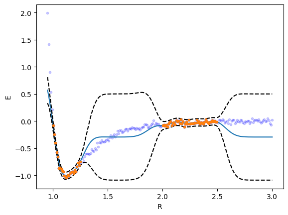
The uncertainty here is primarily related to the model, i.e. it is constrained to be correct where there is data, but with no data, the model is not the right one.
The model does well in the region where there is data, but is qualitatively wrong in the gap (even though classically this would be considered interpolation), and overestimates the uncertainty in this region. The problem is the covariance kernel decays to 0 about two length scales away from the last point, which means there is no data to inform what the weights in that region should look like. That causes the model to revert to the mean of the data.
gpr.predict([[1.8]]), gpr.predict([[3.0]]), np.mean(_y)
| array | ((-0.2452041)) | array | ((-0.29363654)) | -0.2936364964541409 |
Why is this happening? It is not that tricky. You can think of the GP as an expansion of the data in basis functions. The kernel trick effectively makes this expansion in the infinite limit. What are those basis functions? We can draw samples of them, which we show here. You can see that where there is no data, the basis functions are "wiggly". That means they are simply not good at making predictions here.
y_samples = gpr.sample_y(r[:, None], n_samples=15, random_state=0)

plt.plot(r, yp)
plt.plot(r, yp + 2 * se, 'k--', r, yp - 2 * se, 'k--');
plt.plot(_R, _y, '.')

plt.plot(r, y_samples, 'k', alpha=0.2);

plt.xlabel('R')
plt.ylabel('E');

This kernel simply cannot be used for extrapolation, or any predictions more than about two length scales away from the nearest point. Calling it Bayesian doesn't make it better. For similar reasons, this model will not work well outside the data range.
A practical person would still consider using this model, and might even rely on the uncertainty being too large to identify regions of low reliability.
3. a better kernel solves these issues
Not all is lost, if we know more. In this case we can construct a kernel that reflects our understanding that the data came from a Lennard Jones like interaction model. You can construct kernels by adding and multiplying kernels. Here we consider a linear kernel, the DotProduct kernel, and construct a new kernel that is a sum of the linear kernel to the 12th power, a linear kernel to the 6th power, and a WhiteKernel for the noise. It is a little subtle that this kernel should work in \(1 / r\) space, so in addition to kernel engineering, we also do feature engineering.
from sklearn.gaussian_process.kernels import DotProduct

kernel = DotProduct()**12 + DotProduct()**6 +  WhiteKernel()
gpr = GaussianProcessRegressor(kernel=kernel, normalize_y=True).fit(1 / _R, _y)

plt.plot(_R, _y, 'b.')
plt.plot(r, y, 'b.', alpha=0.2)


yp, se = gpr.predict(1 / r[:, None], return_std=True)
plt.plot(r, yp)
plt.plot(r, yp + 2 * se, 'k--', r, yp - 2 * se, 'k--');

plt.xlabel('R')
plt.ylabel('E');

gpr.kernel_
DotProduct(sigma_0=0.0281) ** 12 + DotProduct(sigma_0=0.936) ** 6 + WhiteKernel(noise_level=0.0077)

Note that this GPR does fine in the gap, including the right level of uncertainty there. This model is better because we used the kernel to constrain what forms the model can have. This model actually extrapolates correctly outside the data. It is worth noting that although this model has great predictive and UQ properties, it does not tell us anything about the values of ε and σ in the Lennard Jones model. Although we might say the kernel is physics-based, i.e. it is based on the relevant features and equation, it does not have physical parameters in it.
How about those basis functions here? You can see that all of them basically look like the LJ potential. That means they are good basis functions to expand this data set in.
y_samples = gpr.sample_y(1 / r[:, None], n_samples=15, random_state=0)

plt.plot(_R, _y, '.')

plt.plot(r, y_samples, 'k', alpha=0.2);

plt.xlabel('R')
plt.ylabel('E');

4. How about with feature engineering?
Can we do even better with feature engineering here? Motivated by this comment by Cory Simon, we cast the problem as a linear regression in [1 / r6, 1 / r12] feature space. This is also a perfectly reasonable thing to do. Since our output is linear in these features, we simply use a linear kernel (aka the DotProduct kernel in sklearn).
r6 = 1 / _R**6
r12 = r6**2

kernel = DotProduct() + WhiteKernel()

gpr = GaussianProcessRegressor(kernel=kernel, normalize_y=True).fit(np.hstack([r6, r12]), _y)

plt.plot(_R, _y, 'b.')
plt.plot(r, y, 'b.', alpha=0.2)

fr6 = 1 / r[:, None]**6
fr12 = fr6**2

yp, se = gpr.predict(np.hstack([fr6, fr12]), return_std=True)
plt.plot(r, yp)
plt.plot(r, yp + 2 * se, 'k--', r, yp - 2 * se, 'k--');

plt.xlabel('R')
plt.ylabel('E');

gpr.kernel_
DotProduct(sigma_0=0.74) + WhiteKernel(noise_level=0.00654)

We can't easily plot these basis functions the same way, so we reduce them to a 1-d plot. You can see here that these basis functions practically the same as the one with the advanced kernel.
y_samples = gpr.sample_y(np.hstack([fr6, fr12]),
                         n_samples=15, random_state=0)

plt.plot(_R, _y, '.')

plt.plot(r, y_samples, 'k', alpha=0.2);

plt.xlabel('R')
plt.ylabel('E');

This also works quite well, and is another way to leverage knowledge about what we are building a model for.
5. Summary
Naive use of GPR can provide useful models when you have enough data, but these models likely do not accurately capture uncertainty outside that data, nor is it likely they are reliable in extrapolation. It is possible to do better than this, when you know what to do. Through feature and kernel engineering, you can sometimes create situations where the problem essentially becomes linear regression, where a simple linear kernel is what you want, or you develop a kernel that represents the underlying model. Kernel engineering is generally hard, with limited opportunities to be flexible. See https://www.cs.toronto.edu/~duvenaud/cookbook/ for examples of kernels and combining them.
You can see it is not adequate to say "we used Gaussian process regression". That is about as informative as saying linear regression without identifying the features, or nonlinear regression and not saying what model. You have to be specific about the kernel, and thoughtful about how you know if a prediction is reliable or not. Just because you get an uncertainty prediction doesn't mean its right.
Copyright (C) 2025 by John Kitchin. See the License for information about copying.
Org-mode version = 9.8-pre