The Kitchin Research Group

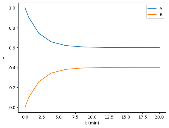
In this example, we aim to find the steady state concentrations of two species by integrating a mass balance to steady state. This is visually easy to see below, the concentrations are essentially flat after 10 min or so. Computationally this is somewhat tricky to find though. A way to do it is to compare some windows of integration to see if the values are not changing very fast. For instance you could average the values from 10 to 11, and compare that to the values in 11 to 12, and keep doing that until they are close enough to the same.

def ode(t, C):
    Ca, Cb = C
    dCadt = -0.2 * Ca + 0.3 * Cb
    dCbdt = -0.3 * Cb + 0.2 * Ca
    return dCadt, dCbdt

tspan = (0, 20)

from scipy.integrate import solve_ivp
sol = solve_ivp(ode, tspan, (1, 0))

import matplotlib.pyplot as plt
plt.plot(sol.t, sol.y.T)
plt.xlabel('t (min)')
plt.ylabel('C')
plt.legend(['A', 'B']);
sol.y.T[-1]

array([0.60003278, 0.39996722])

The goal then is to have a supervisor function that will keep track of the last solution and the current one, and compare the average of them. You could do something more sophisticated, but this is simple enough to try out now. If the difference between two integrations is small enough, we will say we have hit steady state, and if not, we integrate from the end of the last solution forward again. That means we have to store some state information so we can compare a current solution to the last solution.

Let's start by defining a function that returns a solution from some initial condition. Next, we show that if you run it 12ish times, initializing from the last state, we get something that appears steady-stateish in the sense that the y values only changing in the second decimal place. You might consider that close enough to steady state.

def get_sol(C0=(1, 0), window=1):
    sol = solve_ivp(ode, t_span=(0, window), y0=C0)
    return sol

sol = get_sol()
sol = get_sol(sol.y.T[-1])
sol = get_sol(sol.y.T[-1])
sol = get_sol(sol.y.T[-1])
sol = get_sol(sol.y.T[-1])
sol = get_sol(sol.y.T[-1])
sol = get_sol(sol.y.T[-1])
sol = get_sol(sol.y.T[-1])
sol = get_sol(sol.y.T[-1])
sol = get_sol(sol.y.T[-1])
sol = get_sol(sol.y.T[-1])
sol = get_sol(sol.y.T[-1])
sol

  message: The solver successfully reached the end of the integration interval.
  success: True
   status: 0
        t: [ 0.000e+00  3.565e-01  1.000e+00]
        y: [[ 6.016e-01  6.014e-01  6.010e-01]
            [ 3.984e-01  3.986e-01  3.990e-01]]
      sol: None
 t_events: None
 y_events: None
     nfev: 14
     njev: 0
      nlu: 0

That is obviously tedious, so now we devise a supervisor function to do it for us. Since we will save state between calls, I will use a class here. We will define a tolerance that we want the difference of the average of two sequential solutions to be less than. We have to be a little careful here. There are many ways to call get_sol, e.g. all of these are correct, but when the checker function is called, it will get different arguments.

get_sol()           # no args: args=(), kwargs={} 
get_sol((1, 0), 2)  # all positional args: args=((1, 0), 2), kwargs={}
get_sol((1, 0))     # one positional arg:  args=((1, 0),), kwargs={}
get_sol((1, 0), window=2) # a positional and kwarg: args =((1, 0),), kwargs={'window': 2}

We have to either assume one of these, or write a function that can handle any of them. I am going to assume here that args will always just be the initial condition, and anything else will be in kwargs. That is a convention we use for this problem, and if you break the convention, you will have errors. For example, get_sol(C0=(1, 0)) will cause an error because you will not have a positional argument for C0 but instead a keyword argument for C0.

It is not crucial to use a class here; you could also use global variables, or function attributes. A class is a standard way of encapsulating state though. We just have to make the class callable so it acts like a function when we need it to.

class ReachedSteadyState:        
    def __init__(self, tolerance=0.01):
        self.tolerance = tolerance
        self.last_solution = None
        self.count = 0

    def __str__(self):
        return 'ReachedSteadyState'
        
    def __call__(self, args, kwargs, sol):
        if self.last_solution is None:
            self.last_solution = sol
            self.count += 1
            C0 = sol.y.T[-1]
            return (C0,), kwargs

        # we have a previous solution
        if not np.allclose(self.last_solution.y.mean(axis=1),
                           sol.y.mean(axis=1),
                           rtol=self.tolerance,
                           atol=self.tolerance):
            self.last_solution = sol
            self.count += 1
            C0 = sol.y.T[-1]            
            return (C0,), kwargs

Now, we decorate the get_sol function, and then run it. Since we used a bigger window, it only takes 9 iterations to get to an approximate steady state.

def get_sol(C0=(1, 0), window=1):
    sol = solve_ivp(ode, t_span=(0, window), y0=C0)
    return sol

rss = ReachedSteadyState(0.0001)
get_sol = supervisor(check_funcs=(rss,), verbose=True, max_errors=20)(get_sol)
sol = get_sol((1, 0), window=2)
sol

Proposed fix in ReachedSteadyState: ((array([0.74716948, 0.25283052]),), {'window': 2}) Proposed fix in ReachedSteadyState: ((array([0.65414484, 0.34585516]),), {'window': 2}) Proposed fix in ReachedSteadyState: ((array([0.61992776, 0.38007224]),), {'window': 2}) Proposed fix in ReachedSteadyState: ((array([0.60733496, 0.39266504]),), {'window': 2}) Proposed fix in ReachedSteadyState: ((array([0.60269957, 0.39730043]),), {'window': 2}) Proposed fix in ReachedSteadyState: ((array([0.60099346, 0.39900654]),), {'window': 2}) Proposed fix in ReachedSteadyState: ((array([0.60036557, 0.39963443]),), {'window': 2}) Proposed fix in ReachedSteadyState: ((array([0.60013451, 0.39986549]),), {'window': 2}) Proposed fix in ReachedSteadyState: ((array([0.60004949, 0.39995051]),), {'window': 2})

  message: The solver successfully reached the end of the integration interval.
  success: True
   status: 0
        t: [ 0.000e+00  7.179e-01  2.000e+00]
        y: [[ 6.000e-01  6.000e-01  6.000e-01]
            [ 4.000e-01  4.000e-01  4.000e-01]]
      sol: None
 t_events: None
 y_events: None
     nfev: 14
     njev: 0
      nlu: 0

We can plot the two solutions to see how different they are. This shows they are close.

import matplotlib.pyplot as plt
plt.plot(rss.last_solution.t, rss.last_solution.y.T, label=['A previous' ,'B previous'])
plt.plot(sol.t, sol.y.T, '--', label=['A current', 'B current'])
plt.legend()
plt.xlabel('relative t')
plt.ylabel('C');

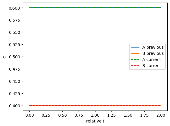
Those look pretty similar on this graph.

Suppose you have a function that randomly fails. This could be because something does not converge with a randomly chosen initial guess, converges to an unphysical answer, etc. In these cases, it makes sense to simply try again with a new initial guess.

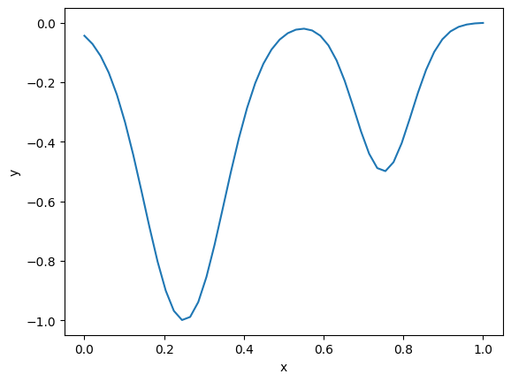
For this example, say we have this objective function with two minima. We will say that any solution above 0.5 is unphysical.

def f(x):
    return -(np.exp(-50 * (x - 0.25)**2) + 0.5 * np.exp(-100 * (x - 0.75)**2))


x = np.linspace(0, 1)
plt.plot(x, f(x))
plt.xlabel('x')
plt.ylabel('y');

Here we define a function that takes a guess, and gets a solution. If the solution is unphysical, we raise an exception. We define a custom exception so we can handle it specifically.

class UnphysicalSolution(Exception):
    pass

def get_minima(guess):
    sol = minimize(f, guess)

    if sol.x > 0.5:
        raise UnphysicalSolution
    else:
        return sol

Some initial guesses work fine.

get_minima(0.2)    

  message: Optimization terminated successfully.
  success: True
   status: 0
      fun: -1.0000000000069416
        x: [ 2.500e-01]
      nit: 4
      jac: [ 4.470e-08]
 hess_inv: [[ 1.000e-02]]
     nfev: 14
     njev: 7

But, others don't.

get_minima(0.8)    

UnphysicalSolution Traceback (most recent call last) Cell In[16], line 1 -—> 1 get_minima(0.8)

Cell In[14], line 8, in get_minima(guess) 5 sol = minimize(f, guess) 7 if sol.x > 0.5: -—> 8 raise UnphysicalSolution 9 else: 10 return sol

UnphysicalSolution:

Here is an example where we can simply rerun with a new guess. That is done here.

def try_again(args, kwargs, exc):
    if isinstance(exc, UnphysicalSolution):
        args = (np.random.random(),)
        return args, kwargs
  
@supervisor(exception_funcs=(try_again,), verbose=True)    
def get_minima(guess):
    sol = minimize(f, guess)

    if sol.x > 0.5:
        raise UnphysicalSolution
    else:
        return sol

get_minima(np.random.random())

Proposed fix in try_again: ((0.7574152313004273,), {})
Proposed fix in try_again: ((0.39650554857922415,), {})
  message: Optimization terminated successfully.
  success: True
   status: 0
      fun: -1.0000000000069411
        x: [ 2.500e-01]
      nit: 3
      jac: [ 0.000e+00]
 hess_inv: [[ 1.000e-02]]
     nfev: 14
     njev: 7

You can see it took two iterations to find a solution. Other times it might take zero or one, or maybe more, it depends on where the guesses fall.

This solution works pretty well, similar to custodian. It is a little simpler than custodian I think, as you can do simple things with functions, and don't really need to make classes for everything. Probably it does less than custodian, and also probably there are some corner issues I haven't uncovered yet. It was a nice exercise in building a decorator though, and thinking through all the ways this can be done.