The Kitchin Research Group

The van der Waal equation of state is:

\(P = \frac{R T}{V - b} - \frac{a}{V^2}\).

We define the reduced pressure as \(P_r = P / P_c\), and the reduced temperature as \(T_r = T / T_c\).

So, we simply solve for V at a given \(P_r\), and then compute \(Z\). There is a subtle trick needed to make this easy to solve, and that is to multiply each side of the equation by \((V - b)\) to avoid a singularity when \(V = b\), which happens in this case near \(P_r \approx 7.5\).

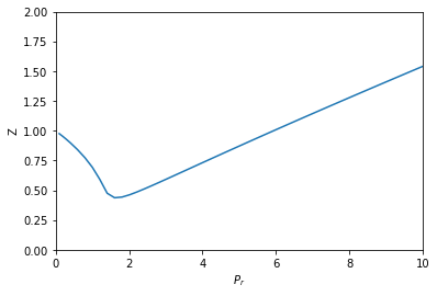
from scipy.optimize import fsolve
import numpy as np
%matplotlib inline
import matplotlib.pyplot as plt

R = 0.08206
Pc = 72.9
Tc = 304.2

a = 27 * R**2 * Tc**2 / (Pc * 64)
b = R * Tc / (8 * Pc)

Tr = 1.1

def objective(V, Pr):
    P = Pr * Pc
    T = Tr * Tc
    return P * (V - b) - (R * T)  +  a / V**2 * (V - b)


Pr_range = np.linspace(0.1, 10)
V = [fsolve(objective, 3, args=(Pr,))[0] for Pr in Pr_range]

T = Tr * Tc
P_range = Pr_range * Pc
Z = P_range * V / (R * T)

plt.plot(Pr_range, Z)
plt.xlabel('$P_r$')
plt.ylabel('Z')
plt.xlim([0, 10])
plt.ylim([0, 2])

(0, 2)

That looks like Figure 7-1 in the book. This approach is fine, but the equation did require a little algebraic finesse to solve, and you have to use some iteration to get the solution.

In this method, you have to derive an expression for \(\frac{dV}{dP_r}\). That derivation goes like this:

\(\frac{dV}{dP_r} = \frac{dV}{dP} \frac{dP}{dP_r}\)

The first term \(\frac{dV}{dP}\) is \((\frac{dP}{dV})^{-1}\), which we can derive directly from the van der Waal equation, and the second term is just a constant: \(P_c\) from the definition of \(P_r\).

They derived:

\(\frac{dP}{dV} = -\frac{R T}{(V - b)^2} + \frac{2 a}{V^3}\)

We need to solve for one V, at the beginning of the range of \(P_r\) we are interested in.

V0, = fsolve(objective, 3, args=(0.1,))
V0

3.6764763125625461

Now, we can define the functions, and integrate them to get the same solution. I defined these pretty verbosely, just for readability.

from scipy.integrate import solve_ivp

def dPdV(V):
    return -R * T / (V - b)**2 + 2 * a / V**3

def dVdP(V):
    return 1 / dPdV(V)

dPdPr = Pc

def dVdPr(Pr, V):
    return dVdP(V) * dPdPr

Pr_span = (0.1, 10)
Pr_eval, h = np.linspace(*Pr_span, retstep=True)

sol = solve_ivp(dVdPr, Pr_span, (V0,), dense_output=True, max_step=h)

V = sol.y[0]
P = sol.t * Pc
Z = P * V / (R * T)
plt.plot(sol.t, Z)
plt.xlabel('$P_r$')
plt.ylabel('Z')
plt.xlim([0, 10])
plt.ylim([0, 2])

(0, 2)

This also looks like Figure 7-1. It is arguably a better approach since we only need an initial condition, and after that have a reliable integration (rather than many iterative solutions from an initial guess of the solution in fsolve).

The only downside to this approach (in my opinion) is the need to derive and implement derivatives. As equations of state get more complex, this gets more tedious and complicated.

The whole point of automatic differentiation is to get derivatives of functions that are written as programs. We explore here the possibility of using this to solve this problem. The idea is to use autograd to define the derivative \(dP/dV\), and then solve the ODE like we did before.

from autograd import grad

def P(V):
    return R * T / (V - b) - a / V**2

# autograd.grad returns a callable that acts like a function
dPdV = grad(P, 0)

def dVdPr(Pr, V):
    return 1 / dPdV(V) * Pc

sol = solve_ivp(dVdPr,  Pr_span, (V0,), dense_output=True, max_step=h)

V, = sol.y
P = sol.t * Pc
Z = P * V / (R * T)
plt.plot(sol.t, Z)
plt.xlabel('$P_r$')
plt.ylabel('Z')
plt.xlim([0, 10])
plt.ylim([0, 2])

(0, 2)

Not surprisingly, this answer looks the same as the previous ones. I think this solution is pretty awesome. We only had to implement the van der Waal equation, and then let autograd do its job to get the relevant derivative. We don't get a free pass on calculus here; we still have to know which derivatives are important. We also need some knowledge about how to use autograd, but with that, this problem becomes pretty easy to solve.