The Kitchin Research Group

In this post we solved a boundary value problem by discretizing it, and approximating the derivatives by finite differences. Here I explore using a neural network to approximate the unknown function, autograd to get the required derivatives, and using autograd to train the neural network to satisfy the differential equations. We will look at the Blasius equation again.

Here I setup a simple neural network

import autograd.numpy as np
from autograd import grad, elementwise_grad
import autograd.numpy.random as npr
from autograd.misc.optimizers import adam

def init_random_params(scale, layer_sizes, rs=npr.RandomState(0)):
    """Build a list of (weights, biases) tuples, one for each layer."""
    return [(rs.randn(insize, outsize) * scale,   # weight matrix
             rs.randn(outsize) * scale)           # bias vector
            for insize, outsize in zip(layer_sizes[:-1], layer_sizes[1:])]


def swish(x):
    "see https://arxiv.org/pdf/1710.05941.pdf"
    return x / (1.0 + np.exp(-x))


def f(params, inputs):
    "Neural network functions"
    for W, b in params:
        outputs = np.dot(inputs, W) + b
        inputs = swish(outputs)    
    return outputs

    
# Here is our initial guess of params:
params = init_random_params(0.1, layer_sizes=[1, 8, 1])

# Derivatives
fp = elementwise_grad(f, 1)
fpp = elementwise_grad(fp, 1)
fppp = elementwise_grad(fpp, 1)

eta = np.linspace(0, 6).reshape((-1, 1))

# This is the function we seek to minimize
def objective(params, step):
    # These should all be zero at the solution
    # f''' + 0.5 f'' f = 0
    zeq = fppp(params, eta) + 0.5 * f(params, eta) * fpp(params, eta) 
    bc0 = f(params, 0.0)  # equal to zero at solution
    bc1 = fp(params, 0.0)  # equal to zero at solution
    bc2 = fp(params, 6.0) - 1.0 # this is the one at "infinity"
    return np.mean(zeq**2) + bc0**2 + bc1**2 + bc2**2

def callback(params, step, g):
    if step % 1000 == 0:
        print("Iteration {0:3d} objective {1}".format(step,
                                                      objective(params, step)))

params = adam(grad(objective), params,
              step_size=0.001, num_iters=10000, callback=callback) 

print('f(0) = {}'.format(f(params, 0.0)))
print('fp(0) = {}'.format(fp(params, 0.0)))
print('fp(6) = {}'.format(fp(params, 6.0)))
print('fpp(0) = {}'.format(fpp(params, 0.0)))

import matplotlib.pyplot as plt
plt.plot(eta, f(params, eta))
plt.xlabel('$\eta$')
plt.ylabel('$f(\eta)$')
plt.xlim([0, 6])
plt.ylim([0, 4.5])
plt.savefig('nn-blasius.png')

Iteration 0 objective 1.11472535 Iteration 1000 objective 0.00049768 Iteration 2000 objective 0.0004579 Iteration 3000 objective 0.00041697 Iteration 4000 objective 0.00037408 Iteration 5000 objective 0.00033705 Iteration 6000 objective 0.00031016 Iteration 7000 objective 0.00029197 Iteration 8000 objective 0.00027585 Iteration 9000 objective 0.00024616 f(0) = -0.00014613 fp(0) = 0.0003518041251639459 fp(6) = 0.999518061473252 fpp(0) = 0.3263370503702663

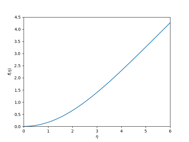I think it is worth discussing what we accomplished here. You can see we have arrived at an approximate solution to our differential equation and the boundary conditions. The boundary conditions seem pretty closely met, and the figure is approximately the same as the previous post. Even better, our solution is an actual function and not a numeric solution that has to be interpolated. We can evaluate it any where we want, including its derivatives!

We did not, however, have to convert the ODE into a system of first-order differential equations, and we did not have to approximate the derivatives with finite differences.

Note, however, that with finite differences we got f''(0)=0.3325. This site reports f''(0)=0.3321. We get close to that here with f''(0) = 0.3263. We could probably get closer to this with more training to reduce the objective function further, or with a finer grid. It is evident that even after 9000 steps, it is still decreasing. Getting accurate derivatives is a stringent test for this, as they are measures of the function curvature.

It is hard to tell how broadly useful this is; I have not tried it beyond this example. In the past, I have found solving BVPs to be pretty sensitive to the initial guesses of the solution. Here we made almost no guess at all, and still got a solution. I find that pretty remarkable.

Copyright (C) 2017 by John Kitchin. See the License for information about copying.

org-mode source

Org-mode version = 9.1.2