The Kitchin Research Group

The Atomic Simulation Environment provides several useful calculators with configurable parameters. For example, the Lennard-Jones potential has two adjustable parameters, σ and ε. I have always thought it would be useful to be able to fit one of these potentials to a reference database, e.g. a DFT database.

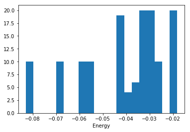
I ran a series of DFT calculations of bulk Ar in different crystal structures, at different volumes and saved them in an ase database (argon.db ). We have five crystal structures at three different volumes. Within each of those sets, I rattled the atoms a bunch of times and calculated the energies. Here is the histogram of energies we have to work with:

%matplotlib inline
import matplotlib.pyplot as plt

import ase.db
db = ase.db.connect('argon.db')

known_energies = [row.energy for row in db.select()]
plt.hist(known_energies, 20)
plt.xlabel('Energy')

What I would really like is a set of Lennard-Jones parameters that describe this data. It only recently occurred to me that we just need to define a function that takes the LJ parameters and computes energies for a set of configurations. Then we create a second objective function we can use in a minimization. Here is how we can implement that idea:

import numpy as np
from scipy.optimize import fmin
from ase.calculators.lj import LennardJones

def my_lj(pars):
    epsilon, sigma = pars
    calc = LennardJones(sigma=sigma, epsilon=epsilon)
    all_atoms = [row.toatoms() for row in db.select()]
    [atoms.set_calculator(calc) for atoms in all_atoms]
    predicted_energies = np.array([atoms.get_potential_energy() for atoms in all_atoms])
    return predicted_energies

def objective(pars):
    known_energies = np.array([row.energy for row in db.select()])
    err = known_energies - my_lj(pars)
    return np.mean(err**2)

LJ_pars = fmin(objective, [0.005, 3.5])        
print(LJ_pars)

Optimization terminated successfully.
         Current function value: 0.000141
         Iterations: 28
         Function evaluations: 53
[ 0.00593014  3.73314611]

Now, let's see how well we do with that fit.

plt.subplot(121)

calc = LennardJones(epsilon=LJ_pars[0], sigma=LJ_pars[1])

for structure, spec in [('fcc', 'b.'),
                        ('hcp', 'r.'),
                        ('bcc', 'g.'),
                        ('diamond', 'gd'),
                        ('sc', 'bs')]:

    ke, pe = [], []
    for row in db.select(structure=structure):
        ke += [row.energy]
        atoms = row.toatoms()
        atoms.set_calculator(calc)
        pe += [atoms.get_potential_energy()]    
    plt.plot(ke, pe, spec, label=structure)

plt.plot([-0.1, 0], [-0.1, 0], 'k-', label='parity')
plt.legend()
plt.xlabel('DFT')
plt.ylabel('LJ')

pred_e = my_lj(LJ_pars)
known_energies = np.array([row.energy for row in db.select()])
err = known_energies - pred_e

plt.subplot(122)
plt.hist(err)
plt.xlabel('error')
plt.tight_layout()

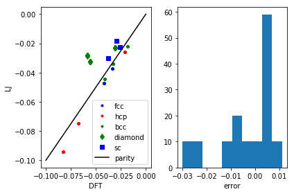
The results aren't fantastic, but you can see that we get the closer packed structures (fcc, hcp, bcc) more accurately than the loosely packed structures (diamond, sc). Those more open structures tend to have more directional bonding, and the Lennard-Jones potential isn't expected to do too well on those. You could consider a more sophisticated model if those structures were important for your simulation.

Copyright (C) 2017 by John Kitchin. See the License for information about copying.

org-mode source

Org-mode version = 9.1.2