Plotting ODE solutions in cylindrical coordinates
Posted February 07, 2013 at 09:00 AM | categories: ode | tags:
Updated March 06, 2013 at 06:33 PM
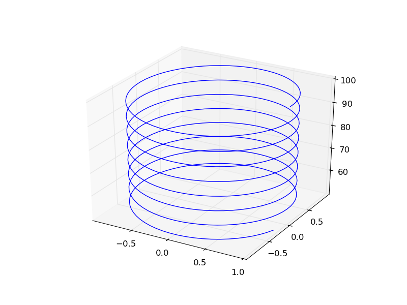
It is straightforward to plot functions in Cartesian coordinates. It is less convenient to plot them in cylindrical coordinates. Here we solve an ODE in cylindrical coordinates, and then convert the solution to Cartesian coordinates for simple plotting.
import numpy as np
from scipy.integrate import odeint

def dfdt(F, t):
    rho, theta, z = F
    drhodt = 0   # constant radius
    dthetadt = 1 # constant angular velocity
    dzdt = -1    # constant dropping velocity
    return [drhodt, dthetadt, dzdt]

# initial conditions
rho0 = 1
theta0 = 0
z0 = 100

tspan = np.linspace(0, 50, 500)
sol = odeint(dfdt, [rho0, theta0, z0], tspan)

rho = sol[:,0]
theta = sol[:,1]
z = sol[:,2]

# convert cylindrical coords to cartesian for plotting.
X = rho * np.cos(theta)
Y = rho * np.sin(theta)

from mpl_toolkits.mplot3d import Axes3D
import matplotlib.pyplot as plt
fig = plt.figure()
ax = fig.gca(projection='3d')
ax.plot(X, Y, z)
plt.savefig('images/ode-cylindrical.png')
Copyright (C) 2013 by John Kitchin. See the License for information about copying.