Modeling a transient plug flow reactor

| categories: pde, animation | tags: reaction engineering

Matlab post

The PDE that describes the transient behavior of a plug flow reactor with constant volumetric flow rate is:

\( \frac{\partial C_A}{\partial dt} = -\nu_0 \frac{\partial C_A}{\partial dV} + r_A \).

To solve this numerically in python, we will utilize the method of lines. The idea is to discretize the reactor in volume, and approximate the spatial derivatives by finite differences. Then we will have a set of coupled ordinary differential equations that can be solved in the usual way. Let us simplify the notation with \(C = C_A\), and let \(r_A = -k C^2\). Graphically this looks like this:

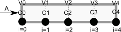
This leads to the following set of equations:

\begin{eqnarray} \frac{dC_0}{dt} &=& 0 \text{ (entrance concentration never changes)} \\ \frac{dC_1}{dt} &=& -\nu_0 \frac{C_1 - C_0}{V_1 - V_0} - k C_1^2 \\ \frac{dC_2}{dt} &=& -\nu_0 \frac{C_2 - C_1}{V_2 - V_1} - k C_2^2 \\ \vdots \\ \frac{dC_4}{dt} &=& -\nu_0 \frac{C_4 - C_3}{V_4 - V_3} - k C_4^2 \end{eqnarray}

Last, we need initial conditions for all the nodes in the discretization. Let us assume the reactor was full of empty solvent, so that \(C_i = 0\) at \(t=0\). In the next block of code, we get the transient solutions, and the steady state solution.

import numpy as np
from scipy.integrate import odeint

Ca0 = 2     # Entering concentration
vo = 2      # volumetric flow rate
volume = 20 # total volume of reactor, spacetime = 10
k = 1       # reaction rate constant

N = 100     # number of points to discretize the reactor volume on

init = np.zeros(N)    # Concentration in reactor at t = 0
init[0] = Ca0         # concentration at entrance

V = np.linspace(0, volume, N) # discretized volume elements
tspan = np.linspace(0, 25)    # time span to integrate over

def method_of_lines(C, t):
    'coupled ODES at each node point'
    D = -vo * np.diff(C) / np.diff(V) - k * C[1:]**2
    return np.concatenate([[0], #C0 is constant at entrance
                            D])


sol = odeint(method_of_lines, init, tspan)

# steady state solution
def pfr(C, V):
    return 1.0 / vo * (-k * C**2)

ssol = odeint(pfr, Ca0, V)

The transient solution contains the time dependent behavior of each node in the discretized reactor. Each row contains the concentration as a function of volume at a specific time point. For example, we can plot the concentration of A at the exit vs. time (that is, the last entry of each row) as:

import matplotlib.pyplot as plt
plt.plot(tspan, sol[:, -1])
plt.xlabel('time')
plt.ylabel('$C_A$ at exit')
plt.savefig('images/transient-pfr-1.png')
[<matplotlib.lines.Line2D object at 0x05A18830>]
<matplotlib.text.Text object at 0x059FE1D0>
<matplotlib.text.Text object at 0x05A05270>

After approximately one space time, the steady state solution is reached at the exit. For completeness, we also examine the steady state solution.

plt.figure()
plt.plot(V, ssol, label='Steady state')
plt.plot(V, sol[-1], label='t = {}'.format(tspan[-1]))
plt.xlabel('Volume')
plt.ylabel('$C_A$')
plt.legend(loc='best')
plt.savefig('images/transient-pfr-2.png')

There is some minor disagreement between the final transient solution and the steady state solution. That is due to the approximation in discretizing the reactor volume. In this example we used 100 nodes. You get better agreement with a larger number of nodes, say 200 or more. Of course, it takes slightly longer to compute then, since the number of coupled odes is equal to the number of nodes.

We can also create an animated gif to show how the concentration of A throughout the reactor varies with time. Note, I had to install ffmpeg (http://ffmpeg.org/) to save the animation.

from matplotlib import animation

# make empty figure
fig = plt.figure()
ax = plt.axes(xlim=(0, 20), ylim=(0, 2))
line, = ax.plot(V, init, lw=2)

def animate(i):
    line.set_xdata(V)
    line.set_ydata(sol[i])
    ax.set_title('t = {0}'.format(tspan[i]))
    ax.figure.canvas.draw() 
    return line,
    

anim = animation.FuncAnimation(fig, animate, frames=50,  blit=True)

anim.save('images/transient_pfr.mp4', fps=10)

http://jkitchin.github.com/media/transient_pfr.mp4

You can see from the animation that after about 10 time units, the solution is not changing further, suggesting steady state has been reached.

Copyright (C) 2013 by John Kitchin. See the License for information about copying.

org-mode source

Discuss on Twitter

Determining linear independence of a set of vectors

| categories: linear algebra | tags: reaction engineering

Matlab post Occasionally we have a set of vectors and we need to determine whether the vectors are linearly independent of each other. This may be necessary to determine if the vectors form a basis, or to determine how many independent equations there are, or to determine how many independent reactions there are.

Reference: Kreysig, Advanced Engineering Mathematics, sec. 7.4

Matlab provides a rank command which gives you the number of singular values greater than some tolerance. The numpy.rank function, unfortunately, does not do that. It returns the number of dimensions in the array. We will just compute the rank from singular value decomposition.

The default tolerance used in Matlab is max(size(A))*eps(norm(A)). Let us break that down. eps(norm(A)) is the positive distance from abs(X) to the next larger in magnitude floating point number of the same precision as X. Basically, the smallest significant number. We multiply that by the size of A, and take the largest number. We have to use some judgment in what the tolerance is, and what “zero” means.

import numpy as np
v1 = [6, 0, 3, 1, 4, 2];
v2 = [0, -1, 2, 7, 0, 5];
v3 = [12, 3, 0, -19, 8, -11];

A = np.row_stack([v1, v2, v3])

# matlab definition
eps = np.finfo(np.linalg.norm(A).dtype).eps
TOLERANCE = max(eps * np.array(A.shape))

U, s, V = np.linalg.svd(A)
print s
print np.sum(s > TOLERANCE)

TOLERANCE = 1e-14
print np.sum(s > TOLERANCE)
>>> >>> >>> >>> >>> >>> ... >>> >>> >>> >>> [  2.75209239e+01   9.30584482e+00   1.42425400e-15]
3
>>> >>> 2

You can see if you choose too small a TOLERANCE, nothing looks like zero. the result with TOLERANCE=1e-14 suggests the rows are not linearly independent. Let us show that one row can be expressed as a linear combination of the other rows.

The number of rows is greater than the rank, so these vectors are not independent. Let's demonstrate that one vector can be defined as a linear combination of the other two vectors. Mathematically we represent this as:

\(x_1 \mathit{v1} + x_2 \mathit{v2} = v3\)

or

\([x_1 x_2][v1; v2] = v3\)

This is not the usual linear algebra form of Ax = b. To get there, we transpose each side of the equation to get:

[v1.T v2.T][x_1; x_2] = v3.T

which is the form Ax = b. We solve it in a least-squares sense.

A = np.column_stack([v1, v2])
x = np.linalg.lstsq(A, v3)
print x[0]
>>> [ 2. -3.]

This shows that v3 = 2*v1 - 3*v2

1 another example

#Problem set 7.4 #17
import numpy as np

v1 = [0.2, 1.2, 5.3, 2.8, 1.6]
v2 = [4.3, 3.4, 0.9, 2.0, -4.3]

A = np.row_stack([v1, v2])
U, s, V = np.linalg.svd(A)
print s
[ 7.57773162  5.99149259]

You can tell by inspection the rank is 2 because there are no near-zero singular values.

2 Near deficient rank

the rank command roughly works in the following way: the matrix is converted to a reduced row echelon form, and then the number of rows that are not all equal to zero are counted. Matlab uses a tolerance to determine what is equal to zero. If there is uncertainty in the numbers, you may have to define what zero is, e.g. if the absolute value of a number is less than 1e-5, you may consider that close enough to be zero. The default tolerance is usually very small, of order 1e-15. If we believe that any number less than 1e-5 is practically equivalent to zero, we can use that information to compute the rank like this.

import numpy as np

A = [[1, 2, 3],
     [0, 2, 3],
     [0, 0, 1e-6]]

U, s, V = np.linalg.svd(A)
print s
print np.sum(np.abs(s) > 1e-15)
print np.sum(np.abs(s) > 1e-5)
[  5.14874857e+00   7.00277208e-01   5.54700196e-07]
3
2

3 Application to independent chemical reactions.

reference: Exercise 2.4 in Chemical Reactor Analysis and Design Fundamentals by Rawlings and Ekerdt.

The following reactions are proposed in the hydrogenation of bromine:

Let this be our species vector: v = [H2 H Br2 Br HBr].T

the reactions are then defined by M*v where M is a stoichometric matrix in which each row represents a reaction with negative stoichiometric coefficients for reactants, and positive stoichiometric coefficients for products. A stoichiometric coefficient of 0 is used for species not participating in the reaction.

import numpy as np

#    [H2  H Br2 Br HBr]
M = [[-1,  0, -1,  0,  2],  # H2 + Br2 == 2HBR
     [ 0,  0, -1,  2,  0],  # Br2 == 2Br
     [-1,  1,  0, -1,  1],  # Br + H2 == HBr + H
     [ 0, -1, -1,  1,  1],  # H + Br2 == HBr + Br
     [ 1, -1,  0,  1,  -1], # H + HBr == H2 + Br
     [ 0,  0,  1, -2,  0]]  # 2Br == Br2

U, s, V = np.linalg.svd(M)
print s
print np.sum(np.abs(s) > 1e-15)

import sympy 
M = sympy.Matrix(M)
reduced_form, inds = M.rref()

print reduced_form

labels = ['H2',  'H', 'Br2', 'Br', 'HBr']
for row in reduced_form.tolist():
    s = '0 = '
    for nu,species in zip(row,labels):
        if nu != 0:
            
            s += ' {0:+d}{1}'.format(int(nu), species)
    if s != '0 = ': print s
[  3.84742803e+00   3.32555975e+00   1.46217301e+00   1.73313660e-16
   8.57422679e-17]
3
[1, 0, 0,  2, -2]
[0, 1, 0,  1, -1]
[0, 0, 1, -2,  0]
[0, 0, 0,  0,  0]
[0, 0, 0,  0,  0]
[0, 0, 0,  0,  0]
0 =  +1H2 +2Br -2HBr
0 =  +1H +1Br -1HBr
0 =  +1Br2 -2Br

6 reactions are given, but the rank of the matrix is only 3. so there are only three independent reactions. You can see that reaction 6 is just the opposite of reaction 2, so it is clearly not independent. Also, reactions 3 and 5 are just the reverse of each other, so one of them can also be eliminated. finally, reaction 4 is equal to reaction 1 minus reaction 3.

There are many possible independent reactions. In the code above, we use sympy to put the matrix into reduced row echelon form, which enables us to identify three independent reactions, and shows that three rows are all zero, i.e. they are not independent of the other three reactions. The choice of independent reactions is not unique.

Copyright (C) 2013 by John Kitchin. See the License for information about copying.

org-mode source

Discuss on Twitter

Conservation of mass in chemical reactions

| categories: linear algebra | tags: reaction engineering

Matlab post

Atoms cannot be destroyed in non-nuclear chemical reactions, hence it follows that the same number of atoms entering a reactor must also leave the reactor. The atoms may leave the reactor in a different molecular configuration due to the reaction, but the total mass leaving the reactor must be the same. Here we look at a few ways to show this.

We consider the water gas shift reaction : \(CO + H_2O \rightleftharpoons H_2 + CO_2\). We can illustrate the conservation of mass with the following equation: \(\bf{\nu}\bf{M}=\bf{0}\). Where \(\bf{\nu}\) is the stoichiometric coefficient vector and \(\bf{M}\) is a column vector of molecular weights. For simplicity, we use pure isotope molecular weights, and not the isotope-weighted molecular weights. This equation simply examines the mass on the right side of the equation and the mass on left side of the equation.

import numpy as np
nu = [-1, -1, 1, 1];
M = [28, 18, 2, 44];
print np.dot(nu, M)
0

You can see that sum of the stoichiometric coefficients times molecular weights is zero. In other words a CO and H_2O have the same mass as H_2 and CO_2.

For any balanced chemical equation, there are the same number of each kind of atom on each side of the equation. Since the mass of each atom is unchanged with reaction, that means the mass of all the species that are reactants must equal the mass of all the species that are products! Here we look at the number of C, O, and H on each side of the reaction. Now if we add the mass of atoms in the reactants and products, it should sum to zero (since we used the negative sign for stoichiometric coefficients of reactants).

import numpy as np
            # C   O   H
reactants = [-1, -2, -2]
products  = [ 1,  2,  2]

atomic_masses = [12.011, 15.999, 1.0079]  # atomic masses

print np.dot(reactants, atomic_masses) + np.dot(products, atomic_masses)
>>> ... >>> >>> >>> >>> >>> 0.0

That is all there is to mass conservation with reactions. Nothing changes if there are lots of reactions, as long as each reaction is properly balanced, and none of them are nuclear reactions!

Copyright (C) 2013 by John Kitchin. See the License for information about copying.

org-mode source

Discuss on Twitter

The Gibbs free energy of a reacting mixture and the equilibrium composition

| categories: optimization | tags: reaction engineering, thermodynamics

Table of Contents

Matlab post

In this post we derive the equations needed to find the equilibrium composition of a reacting mixture. We use the method of direct minimization of the Gibbs free energy of the reacting mixture.

The Gibbs free energy of a mixture is defined as \(G = \sum\limits_j \mu_j n_j\) where \(\mu_j\) is the chemical potential of species \(j\), and it is temperature and pressure dependent, and \(n_j\) is the number of moles of species \(j\).

We define the chemical potential as \(\mu_j = G_j^\circ + RT\ln a_j\), where \(G_j^\circ\) is the Gibbs energy in a standard state, and \(a_j\) is the activity of species \(j\) if the pressure and temperature are not at standard state conditions.

If a reaction is occurring, then the number of moles of each species are related to each other through the reaction extent \(\epsilon\) and stoichiometric coefficients: \(n_j = n_{j0} + \nu_j \epsilon\). Note that the reaction extent has units of moles.

Combining these three equations and expanding the terms leads to:

$$G = \sum\limits_j n_{j0}G_j^\circ +\sum\limits_j \nu_j G_j^\circ \epsilon +RT\sum\limits_j(n_{j0} + \nu_j\epsilon)\ln a_j $$

The first term is simply the initial Gibbs free energy that is present before any reaction begins, and it is a constant. It is difficult to evaluate, so we will move it to the left side of the equation in the next step, because it does not matter what its value is since it is a constant. The second term is related to the Gibbs free energy of reaction: \(\Delta_rG = \sum\limits_j \nu_j G_j^\circ\). With these observations we rewrite the equation as:

$$G - \sum\limits_j n_{j0}G_j^\circ = \Delta_rG \epsilon +RT\sum\limits_j(n_{j0} + \nu_j\epsilon)\ln a_j $$

Now, we have an equation that allows us to compute the change in Gibbs free energy as a function of the reaction extent, initial number of moles of each species, and the activities of each species. This difference in Gibbs free energy has no natural scale, and depends on the size of the system, i.e. on \(n_{j0}\). It is desirable to avoid this, so we now rescale the equation by the total initial moles present, \(n_{T0}\) and define a new variable \(\epsilon' = \epsilon/n_{T0}\), which is dimensionless. This leads to:

$$ \frac{G - \sum\limits_j n_{j0}G_j^\circ}{n_{T0}} = \Delta_rG \epsilon' + RT \sum\limits_j(y_{j0} + \nu_j\epsilon')\ln a_j $$

where \(y_{j0}\) is the initial mole fraction of species \(j\) present. The mole fractions are intensive properties that do not depend on the system size. Finally, we need to address \(a_j\). For an ideal gas, we know that \(A_j = \frac{y_j P}{P^\circ}\), where the numerator is the partial pressure of species \(j\) computed from the mole fraction of species \(j\) times the total pressure. To get the mole fraction we note:

$$y_j = \frac{n_j}{n_T} = \frac{n_{j0} + \nu_j \epsilon}{n_{T0} + \epsilon \sum\limits_j \nu_j} = \frac{y_{j0} + \nu_j \epsilon'}{1 + \epsilon'\sum\limits_j \nu_j} $$

This finally leads us to an equation that we can evaluate as a function of reaction extent:

$$ \frac{G - \sum\limits_j n_{j0}G_j^\circ}{n_{T0}} = \widetilde{\widetilde{G}} = \Delta_rG \epsilon' + RT\sum\limits_j(y_{j0} + \nu_j\epsilon') \ln\left(\frac{y_{j0}+\nu_j\epsilon'}{1+\epsilon'\sum\limits_j\nu_j} \frac{P}{P^\circ}\right) $$

we use a double tilde notation to distinguish this quantity from the quantity derived by Rawlings and Ekerdt which is further normalized by a factor of \(RT\). This additional scaling makes the quantities dimensionless, and makes the quantity have a magnitude of order unity, but otherwise has no effect on the shape of the graph.

Finally, if we know the initial mole fractions, the initial total pressure, the Gibbs energy of reaction, and the stoichiometric coefficients, we can plot the scaled reacting mixture energy as a function of reaction extent. At equilibrium, this energy will be a minimum. We consider the example in Rawlings and Ekerdt where isobutane (I) reacts with 1-butene (B) to form 2,2,3-trimethylpentane (P). The reaction occurs at a total pressure of 2.5 atm at 400K, with equal molar amounts of I and B. The standard Gibbs free energy of reaction at 400K is -3.72 kcal/mol. Compute the equilibrium composition.

import numpy as np

R = 8.314
P = 250000  # Pa
P0 = 100000 # Pa, approximately 1 atm
T = 400 # K

Grxn = -15564.0 #J/mol
yi0 = 0.5; yb0 = 0.5; yp0 = 0.0; # initial mole fractions

yj0 = np.array([yi0, yb0, yp0])
nu_j = np.array([-1.0, -1.0, 1.0])   # stoichiometric coefficients

def Gwigglewiggle(extentp):
    diffg = Grxn * extentp
    sum_nu_j = np.sum(nu_j)
    for i,y in enumerate(yj0):
        x1 = yj0[i] + nu_j[i] * extentp
        x2 = x1 / (1.0 + extentp*sum_nu_j)
        diffg += R * T * x1 * np.log(x2 * P / P0)
    return diffg

There are bounds on how large \(\epsilon'\) can be. Recall that \(n_j = n_{j0} + \nu_j \epsilon\), and that \(n_j \ge 0\). Thus, \(\epsilon_{max} = -n_{j0}/\nu_j\), and the maximum value that \(\epsilon'\) can have is therefore \(-y_{j0}/\nu_j\) where \(y_{j0}>0\). When there are multiple species, you need the smallest \(epsilon'_{max}\) to avoid getting negative mole numbers.

epsilonp_max = min(-yj0[yj0 > 0] / nu_j[yj0 > 0])
epsilonp = np.linspace(1e-6, epsilonp_max, 1000);

import matplotlib.pyplot as plt

plt.plot(epsilonp,Gwigglewiggle(epsilonp))
plt.xlabel('$\epsilon$')
plt.ylabel('Gwigglewiggle')
plt.savefig('images/gibbs-minim-1.png')
>>> >>> >>> __main__:7: RuntimeWarning: divide by zero encountered in log
__main__:7: RuntimeWarning: invalid value encountered in multiply
[<matplotlib.lines.Line2D object at 0x10b1c7710>]
<matplotlib.text.Text object at 0x10b1c3d10>
<matplotlib.text.Text object at 0x10b1c9b90>

Now we simply minimize our Gwigglewiggle function. Based on the figure above, the miminum is near 0.45.

from scipy.optimize import fminbound

epsilonp_eq = fminbound(Gwigglewiggle, 0.4, 0.5)
print epsilonp_eq

plt.plot([epsilonp_eq], [Gwigglewiggle(epsilonp_eq)], 'ro')
plt.savefig('images/gibbs-minim-2.png')
>>> >>> 0.46959618249
>>> [<matplotlib.lines.Line2D object at 0x10d4d3e50>]

To compute equilibrium mole fractions we do this:

yi = (yi0 + nu_j[0]*epsilonp_eq) / (1.0 + epsilonp_eq*np.sum(nu_j))
yb = (yb0 + nu_j[1]*epsilonp_eq) / (1.0 + epsilonp_eq*np.sum(nu_j))
yp = (yp0 + nu_j[2]*epsilonp_eq) / (1.0 + epsilonp_eq*np.sum(nu_j))

print yi, yb, yp

# or this
y_j = (yj0 + np.dot(nu_j, epsilonp_eq)) / (1.0 + epsilonp_eq*np.sum(nu_j))
print y_j
>>> >>> >>> 0.0573220186324 0.0573220186324 0.885355962735
>>> ... >>> [ 0.05732202  0.05732202  0.88535596]

\(K = \frac{a_P}{a_I a_B} = \frac{y_p P/P^\circ}{y_i P/P^\circ y_b P/P^\circ} = \frac{y_P}{y_i y_b}\frac{P^\circ}{P}\).

We can express the equilibrium constant like this :\(K = \prod\limits_j a_j^{\nu_j}\), and compute it with a single line of code.

K = np.exp(-Grxn/R/T)
print 'K from delta G ',K
print 'K as ratio of mole fractions ',yp / (yi * yb) * P0 / P
print 'compact notation: ',np.prod((y_j * P / P0)**nu_j)
K from delta G  107.776294742
K as ratio of mole fractions  107.779200065
compact notation:  107.779200065

These results are very close, and only disagree because of the default tolerance used in identifying the minimum of our function. You could tighten the tolerances by setting options to the fminbnd function.

1 Summary

In this post we derived an equation for the Gibbs free energy of a reacting mixture and used it to find the equilibrium composition. In future posts we will examine some alternate forms of the equations that may be more useful in some circumstances.

Copyright (C) 2014 by John Kitchin. See the License for information about copying.

org-mode source

Org-mode version = 8.2.7c

Discuss on Twitter

Plug flow reactor with a pressure drop

| categories: ode | tags: reaction engineering, fluids

If there is a pressure drop in a plug flow reactor, 1 there are two equations needed to determine the exit conversion: one for the conversion, and one from the pressure drop.

\begin{eqnarray} \frac{dX}{dW} &=& \frac{k'}{F_A0} \left ( \frac{1-X}{1 + \epsilon X} \right) y\\ \frac{dX}{dy} &=& -\frac{\alpha (1 + \epsilon X)}{2y} \end{eqnarray}

Here is how to integrate these equations numerically in python.

import numpy as np
from scipy.integrate import odeint
import matplotlib.pyplot as plt

kprime = 0.0266
Fa0 = 1.08
alpha = 0.0166
epsilon = -0.15

def dFdW(F, W):
    'set of ODEs to integrate'
    X = F[0]
    y = F[1]
    dXdW = kprime / Fa0 * (1-X) / (1 + epsilon*X) * y
    dydW = -alpha * (1 + epsilon * X) / (2 * y)
    return [dXdW, dydW]

Wspan = np.linspace(0,60)
X0 = 0.0
y0 = 1.0
F0 = [X0, y0]
sol = odeint(dFdW, F0, Wspan)

# now plot the results
plt.plot(Wspan, sol[:,0], label='Conversion')
plt.plot(Wspan, sol[:,1], 'g--', label='y=$P/P_0$')
plt.legend(loc='best')
plt.xlabel('Catalyst weight (lb_m)')
plt.savefig('images/2013-01-08-pdrop.png')

Here is the resulting figure.

Copyright (C) 2013 by John Kitchin. See the License for information about copying.

org-mode source

Discuss on Twitter
Next Page ยป