Training the ASE Lennard-Jones potential to DFT calculations

| categories: autograd, python | tags:

The Atomic Simulation Environment provides several useful calculators with configurable parameters. For example, the Lennard-Jones potential has two adjustable parameters, σ and ε. I have always thought it would be useful to be able to fit one of these potentials to a reference database, e.g. a DFT database.

I ran a series of DFT calculations of bulk Ar in different crystal structures, at different volumes and saved them in an ase database (argon.db ). We have five crystal structures at three different volumes. Within each of those sets, I rattled the atoms a bunch of times and calculated the energies. Here is the histogram of energies we have to work with:

%matplotlib inline
import matplotlib.pyplot as plt

import ase.db
db = ase.db.connect('argon.db')

known_energies = [row.energy for row in db.select()]
plt.hist(known_energies, 20)
plt.xlabel('Energy')

What I would really like is a set of Lennard-Jones parameters that describe this data. It only recently occurred to me that we just need to define a function that takes the LJ parameters and computes energies for a set of configurations. Then we create a second objective function we can use in a minimization. Here is how we can implement that idea:

import numpy as np
from scipy.optimize import fmin
from ase.calculators.lj import LennardJones

def my_lj(pars):
    epsilon, sigma = pars
    calc = LennardJones(sigma=sigma, epsilon=epsilon)
    all_atoms = [row.toatoms() for row in db.select()]
    [atoms.set_calculator(calc) for atoms in all_atoms]
    predicted_energies = np.array([atoms.get_potential_energy() for atoms in all_atoms])
    return predicted_energies

def objective(pars):
    known_energies = np.array([row.energy for row in db.select()])
    err = known_energies - my_lj(pars)
    return np.mean(err**2)

LJ_pars = fmin(objective, [0.005, 3.5])        
print(LJ_pars)
Optimization terminated successfully.
         Current function value: 0.000141
         Iterations: 28
         Function evaluations: 53
[ 0.00593014  3.73314611]

Now, let's see how well we do with that fit.

plt.subplot(121)

calc = LennardJones(epsilon=LJ_pars[0], sigma=LJ_pars[1])

for structure, spec in [('fcc', 'b.'),
                        ('hcp', 'r.'),
                        ('bcc', 'g.'),
                        ('diamond', 'gd'),
                        ('sc', 'bs')]:

    ke, pe = [], []
    for row in db.select(structure=structure):
        ke += [row.energy]
        atoms = row.toatoms()
        atoms.set_calculator(calc)
        pe += [atoms.get_potential_energy()]    
    plt.plot(ke, pe, spec, label=structure)

plt.plot([-0.1, 0], [-0.1, 0], 'k-', label='parity')
plt.legend()
plt.xlabel('DFT')
plt.ylabel('LJ')

pred_e = my_lj(LJ_pars)
known_energies = np.array([row.energy for row in db.select()])
err = known_energies - pred_e

plt.subplot(122)
plt.hist(err)
plt.xlabel('error')
plt.tight_layout()

The results aren't fantastic, but you can see that we get the closer packed structures (fcc, hcp, bcc) more accurately than the loosely packed structures (diamond, sc). Those more open structures tend to have more directional bonding, and the Lennard-Jones potential isn't expected to do too well on those. You could consider a more sophisticated model if those structures were important for your simulation.

Copyright (C) 2017 by John Kitchin. See the License for information about copying.

org-mode source

Org-mode version = 9.1.2

Discuss on Twitter

Neural networks for regression with autograd

| categories: autograd, python | tags:

Today we are going to take a meandering path to using autograd to train a neural network for regression. First let's consider this very general looking nonlinear model that we might fit to data. There are 10 parameters in it, so we should expect we can get it to fit some data pretty well.

\(y = b1 + w10 tanh(w00 x + b00) + w11 tanh(w01 x + b01) + w12 tanh(w02 x + b02)\)

We will use it to fit data that is generated from \(y = x^\frac{1}{3}\). First, we just do a least_squares fit. This function can take a jacobian function, so we provide one using autograd.

import autograd.numpy as np
from autograd import jacobian

from scipy.optimize import curve_fit

# Some generated data
X = np.linspace(0, 1)
Y = X**(1. / 3.)

def model(x, *pars):
    b1, w10, w00, b00, w11, w01, b01, w12, w02, b02 = pars
    pred = b1 + w10 * np.tanh(w00 * x + b00) + w11 * np.tanh(w01 * x + b01) + w12 * np.tanh(w02 * x + b02)
    return pred


def resid(pars):
    return Y - model(X, *pars)
MSE:  0.0744600049689

We will look at some timing of this regression. Here we do not provide a jacobian.

%%timeit
pars = least_squares(resid, np.random.randn(10)*0.1).x
1.21 s ± 42.7 ms per loop (mean ± std. dev. of 7 runs, 1 loop each)

And here we do provide one. It takes a lot longer to do this. We do have a jacobian of 10 parameters, so that ends up being a lot of extra computations to do.

%%timeit
pars = least_squares(resid, np.random.randn(10)*0.1, jac=jacobian(resid)).x
24.1 s ± 1.61 s per loop (mean ± std. dev. of 7 runs, 1 loop each)

We will print these parameters for reference later.

b1, w10, w00, b00, w11, w01, b01, w12, w02, b02 = pars

print([w00, w01, w02], [b00, b01, b02])
print([w10, w11, w12], b1)
[5.3312122926210703, 54.6923797622945, -0.50881373227993232] [2.9834159679095662, 2.6062295455987199, -2.3782572250527778]
[42.377172168160477, 22.036104340171004, -50.075636975961089] -113.179935862

Let's just make sure the fit looks ok. I am going to plot it outside the fitted region to see how it extrapolates. The shaded area shows the region we did the fitting in.

X2 = np.linspace(0, 3)
Y2 = X2**(1. / 3.)

Z2 = model(X2, *pars)

plt.plot(X2, Y2, 'b.', label='analytical')
plt.plot(X2, Z2, label='model')
plt.fill_between(X2 < 1, 0, 1.4, facecolor='gray', alpha=0.5)

You can seen it fits pretty well from 0 to 1 where we fitted it, but outside that the model is not accurate. Our model is not that related to the true function of the model, so there is no reason to expect it should extrapolate.

I didn't pull that model out of nowhere. Let's rewrite it in a few steps. If we think of tanh as a function that operates element-wise on a vector, we could write that equation more compactly at:

                              [w00 * x + b01] 
y = [w10, w11, w12] @ np.tanh([w01 * x + b01]) + b1
                              [w02 * x + b02]  

We can rewrite this one more time in matrix notation:

y = w1 @ np.tanh(w0 @ x + b0) + b1

Another way to read these equations is that we have an input of x. We multiply the input by a vector weights (w0), add a vector of offsets (biases), b0, activate that by the nonlinear tanh function, then multiply that by a new set of weights, and add a final bias. We typically call this kind of model a neural network. There is an input layer, one hidden layer with 3 neurons that are activated by tanh, and one output layer with linear activation.

Autograd was designed in part for building neural networks. In the next part of this post, we reformulate this regression as a neural network. This code is lightly adapted from https://github.com/HIPS/autograd/blob/master/examples/neural_net_regression.py.

The first function initializes the weights and biases for each layer in our network. It is standard practice to initialize them to small random numbers to avoid any unintentional symmetries that might occur from a systematic initialization (e.g. all ones or zeros). The second function sets up the neural network and computes its output.

from autograd import grad
import autograd.numpy.random as npr
from autograd.misc.optimizers import adam

def init_random_params(scale, layer_sizes, rs=npr.RandomState(0)):
    """Build a list of (weights, biases) tuples, one for each layer."""
    return [(rs.randn(insize, outsize) * scale,   # weight matrix
             rs.randn(outsize) * scale)           # bias vector
            for insize, outsize in zip(layer_sizes[:-1], layer_sizes[1:])]

def nn_predict(params, inputs, activation=np.tanh):
    for W, b in params[:-1]:
        outputs = np.dot(inputs, W) + b
        inputs = activation(outputs)
    # no activation on the last layer
    W, b = params[-1]
    return np.dot(inputs, W) + b

Here we use the first function to define the weights and biases for a neural network with one input, one hidden layer of 3 neurons, and one output layer.

init_scale = 0.1
    
# Here is our initial guess:
params = init_random_params(init_scale, layer_sizes=[1, 3, 1])
for i, wb in enumerate(params):
    W, b = wb
    print('w{0}: {1}, b{0}: {2}'.format(i, W.shape, b.shape))
w0: (1, 3), b0: (3,)
w1: (3, 1), b1: (1,)

You can see w0 is a column vector of weights, and there are three biases in b0. W1 in contrast, is a row vector of weights, with one bias. So 10 parameters in total, like we had before. We will create an objective function of the mean squared error again, and a callback function to show us the progress.

Then we run the optimization step iteratively until we get our objective function below a tolerance we define.

def objective(params, _):
    pred = nn_predict(params, X.reshape([-1, 1]))
    err = Y.reshape([-1, 1]) - pred
    return np.mean(err**2)


def callback(params, step, g):
    if step % 250 == 0:
        print("Iteration {0:3d} objective {1:1.2e}".format(i * N + step,
                                                           objective(params, step)))

N = 500
NMAX = 20

for i in range(NMAX):
    params = adam(grad(objective), params,
                  step_size=0.01, num_iters=N, callback=callback)
    if objective(params, _) < 2e-5:
        break
Iteration   0 objective 5.30e-01
Iteration 250 objective 4.52e-03
Iteration 500 objective 4.17e-03
Iteration 750 objective 1.86e-03
Iteration 1000 objective 1.63e-03
Iteration 1250 objective 1.02e-03
Iteration 1500 objective 6.30e-04
Iteration 1750 objective 4.54e-04
Iteration 2000 objective 3.25e-04
Iteration 2250 objective 2.34e-04
Iteration 2500 objective 1.77e-04
Iteration 2750 objective 1.35e-04
Iteration 3000 objective 1.04e-04
Iteration 3250 objective 7.86e-05
Iteration 3500 objective 5.83e-05
Iteration 3750 objective 4.46e-05
Iteration 4000 objective 3.39e-05
Iteration 4250 objective 2.66e-05
Iteration 4500 objective 2.11e-05
Iteration 4750 objective 1.71e-05

Let's compare these parameters to the previous ones we got.

for i, wb in enumerate(params):
    W, b = wb
    print('w{0}: {1}, b{0}: {2}'.format(i, W, b))
w0: [[ -0.71332351   3.23209728 -32.51135373]], b0: [ 0.45819205  0.19314303 -0.8687    ]
w1: [[-0.53699549]
 [ 0.39522207]
 [-1.05457035]], b1: [-0.58005452]

These look pretty different. It is not too surprising that there could be more than one set of these parameters that give similar fits. The original data only requires two parameters to create it: \(y = a x^b\), where \(x=1\) and \(b=1/3\). We have 8 extra parameters of flexibility in this model.

Let's again examine the fit of our model to the data.

Z2 = nn_predict(params, X2.reshape([-1, 1]))

plt.plot(X2, Y2, 'b.', label='analytical')
plt.plot(X2, Z2, label='NN')
plt.fill_between(X2 < 1, 0, 1.4, facecolor='gray', alpha=0.5)

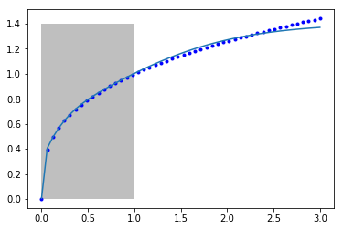
Once again, we can see that between 0 and 1 where the model was fitted we get a good fit, but past that the model does not fit the known function well. It is coincidentally better than our previous model, but as before it is not advisable to use this model for extrapolation. Even though we say it "learned" something about the data, it clearly did not learn the function \(y=x^{1/3}\). It did "learn" some approximation to it in the region of x=0 to 1. Of course, it did not learn anything that the first nonlinear regression model didn't learn.

Now you know the secret of a neural network, it is just a nonlinear model. Without the activation, it is just a linear model. So, why use linear regression, when you can use an unactivated neural network and call it AI?

Copyright (C) 2017 by John Kitchin. See the License for information about copying.

org-mode source

Org-mode version = 9.1.2

Discuss on Twitter

Using autograd in nonlinear regression

| categories: regression, autograd, python | tags:

Table raw-data contains the energy as a function of volume for some solid material from a set of density functional theory calculations. Our goal is to fit the Murnaghan equation of state to this data. The model is moderately nonlinear. I have previously done this with the standard nonlinear regression functions in scipy, so today we will use autograd along with a builtin optimizer to minimize an objective function to achieve the same thing.

The basic idea is we define an objective function, in this case the summed squared errors between predicted values from the model and known values from our data. The objective function takes two arguments: the model parameters, and the "step". This function signature is a consequence of the built in optimizer we use; it expects that signature (it is useful for batch training, but we will not use that here). We use autograd to create a gradient of the objective function which the adam optimizer will use to vary the parameters with the goal of minimizing the objective function.

The adam optimizer function takes as one argument a callback function, which we call summary to print out intermediate results during the convergence. We run the optimizer in a loop because the optimizer runs a fixed number of steps on each call. We check if the objective function is sufficiently small, and if it is we break out.

import autograd.numpy as np
from autograd import grad
from autograd.misc.optimizers import adam

np.set_printoptions(precision=3, suppress=True)

# input data
Vinput = np.array([row[0] for row in data]) 
Eknown = np.array([row[1] for row in data])

def Murnaghan(pars, vol):
    '''
    given a vector of parameters and volumes, return a vector of energies.
    equation From PRB 28,5480 (1983)
    '''
    E0, B0, BP, V0 = pars
    E = E0 + B0 * vol / BP * (((V0 / vol)**BP) / (BP - 1.0) + 1.0) - V0 * B0 / (BP - 1.)
    return E

def objective(pars, step):
    "This is what we want to minimize by varying the pars."
    predicted = Murnaghan(pars, Vinput)
    # Note Eknown is not defined in this function scope
    errors = Eknown - predicted
    return np.sum(errors**2)

objective_grad = grad(objective)

def summary(pars, step, gradient):
    # Note i, N are not defined in this function scope
    if step % N == 0: 
        print('step {0:5d}: {1:1.3e}'.format(i * N + step, 
                                             objective(pars, step)))

pars = np.array([-400, 0.5, 2, 210]) # The initial guess
N = 200 # num of steps to take on each optimization
learning_rate = 0.001
for i in range(100):
    pars = adam(objective_grad, pars, step_size=learning_rate, 
                num_iters=N, callback=summary)
    SSE = objective(pars, None)
    if SSE < 0.00002:
        print('Tolerance met.', SSE)
        break
print(pars)
step     0: 3.127e+02
step   200: 1.138e+02
step   400: 2.011e+01
step   600: 1.384e+00
step   800: 1.753e-01
step  1000: 2.044e-03
step  1200: 1.640e-03
step  1400: 1.311e-03
step  1600: 1.024e-03
step  1800: 7.765e-04
step  2000: 5.698e-04
step  2200: 4.025e-04
step  2400: 2.724e-04
step  2600: 1.762e-04
step  2800: 1.095e-04
step  3000: 6.656e-05
step  3200: 3.871e-05
step  3400: 2.359e-05
('Tolerance met.', 1.5768901008364176e-05)
[-400.029    0.004    4.032  211.847]

There are some subtleties in the code above. One is the variables that are used kind of all over the place, which is noted in a few places. Those could get tricky to keep track of. Another is the variable I called learning_rate. I borrowed that terminology from the machine learning community. It is the step_size in this implementation of the optimizer. If you make it too large, the objective function doesn't converge, but if you set it too small, it will take a long time to converge. Note that it took at about 3400 steps of "training". This is a lot more than is typically required by something like pycse.nlinfit. This isn't the typical application for this approach to regression. More on that another day.

As with any fit, it is wise to check it out at least graphically. Here is the fit and data.

%matplotlib inline
import matplotlib
matplotlib.rc('axes.formatter', useoffset=False)
import matplotlib.pyplot as plt

plt.plot(Vinput, Eknown, 'ko', label='known')

vinterp = np.linspace(Vinput.min(), Vinput.max(), 200)

plt.plot(vinterp, Murnaghan(pars, vinterp), 'r-', label='predicted')
plt.xlabel('Vol')
plt.ylabel('E')

The fit looks pretty good.

Table 1: Volume-Energy data for a solid state system.
volume energy
324.85990899 -399.9731688470
253.43999457 -400.0172393178
234.03826687 -400.0256270548
231.12159387 -400.0265690700
228.40609504 -400.0273551120
225.86490337 -400.0280030862
223.47556626 -400.0285313450
221.21992353 -400.0289534593
219.08319566 -400.0292800709
217.05369547 -400.0295224970
215.12089909 -400.0296863867
213.27525144 -400.0297809256
211.51060823 -400.0298110000
203.66743321 -400.0291665573
197.07888649 -400.0275017142
191.39717952 -400.0250998136
186.40163591 -400.0221371852
181.94435510 -400.0187369863
177.92077043 -400.0149820198
174.25380090 -400.0109367042
170.88582166 -400.0066495100
167.76711189 -400.0021478258
164.87096104 -399.9974753449
159.62553397 -399.9876885136
154.97005460 -399.9774175487
150.78475335 -399.9667603369
146.97722201 -399.9557686286
143.49380641 -399.9445262604

Copyright (C) 2017 by John Kitchin. See the License for information about copying.

org-mode source

Org-mode version = 9.1.2

Discuss on Twitter

Sensitivity analysis using automatic differentiation in Python

| categories: autograd, python, sensitivity | tags:

This paper describes how sensitivity analysis requires access to the derivatives of a function. Say, for example we have a function describing the time evolution of the concentration of species A:

\([A] = \frac{[A]_0}{k_1 + k_{-1}} (k_1 e^{(-(k_1 _ k_{-1})t)} + k_{-1})\)

The local sensitivity of the concentration of A to the parameters \(k1\) and \(k_1\) are defined as \(\frac{\partial A}{\partial k1}\) and \(\frac{\partial A}{\partial k_1}\). Our goal is to plot the sensitivity as a function of time. We could derive those derivatives, but we will use auto-differentiation instead through the autograd package. Here we import numpy from the autograd package and plot the function above.

import autograd.numpy as np

A0 = 1.0

def A(t, k1, k_1):
    return A0 / (k1 + k_1) * (k1 * np.exp(-(k1 + k_1) * t) + k_1)

%matplotlib inline
import matplotlib.pyplot as plt

t = np.linspace(0, 0.5)

k1 = 3.0
k_1 = 3.0
plt.plot(t, A(t, k1, k_1))
plt.xlim([0, 0.5])
plt.ylim([0, 1])
plt.xlabel('t')
plt.ylabel('A')

The figure above reproduces Fig. 1 from the paper referenced above. Next, we use autograd to get the derivatives. This is subtly different than our previous post. First, we need the derivative of the function with respect to the second and third arguments; the default is the first argument. Second, we want to evaluate this derivative at each time value. We use the jacobian function in autograd to get these. This is different than grad, which will sum up the derivatives at each time. That might be useful for regression, but not for sensitivity analysis. Finally, to reproduce Figure 2a, we plot the absolute value of the sensitivities.

from autograd import jacobian

dAdk1 = jacobian(A, 1)
dAdk_1 = jacobian(A, 2)

plt.plot(t, np.abs(dAdk1(t, k1, k_1)))
plt.plot(t, np.abs(dAdk_1(t, k1, k_1)))
plt.xlim([0, 0.5])
plt.ylim([0, 0.1])
plt.xlabel('t')
plt.legend(['$S_{k1}$', '$S_{k\_1}$'])

That looks like the figure in the paper. To summarize the main takeaway, autograd enabled us to readily compute derivatives without having to derive them manually. There was a little subtlety in choosing jacobian over grad or elementwise_grad but once you know what these do, it seems reasonable. It is important to import the wrapped numpy first, to enable autograd to do its work. All the functions here are pretty standard, so everything worked out of the box. We should probably be using autograd, or something like it for more things in science!

Copyright (C) 2017 by John Kitchin. See the License for information about copying.

org-mode source

Org-mode version = 9.1.2

Discuss on Twitter

A Hy macro for defining functions with docstrings on each argument

| categories: hylang, python | tags:

For functions with a lot of arguments, python style docstrings leave something to be desired. For one, they are not that close to the arguments, so if you have a function with say 20 arguments, the docstring might take up a whole page! That means they are hard to keep synchronized too. Let's not argue now over the merits of a function with 20+ arguments, it is enough that they exist, and are a problem.

So what are typical documentation standards? Here is a Numpy style doc string:

def func(arg1, arg2):
    """multiply arg1 and arg2

    Parameters
    ----------
    arg1 : a number
    arg2 : a number

    """
    return arg1 * arg2

It works well for a small number of arguments with limited descriptions. This is a proper docstring that is accessible by introspection and pydoc. With much longer argument lists, this falls apart. I will not pick on any code in particular here, but suffice it to say I was inspired today to think of a better way. There are some other documentation solutions at http://stackoverflow.com/questions/9195455/how-to-document-a-method-with-parameters, but None of them are better in my opinion. I want accessible docstrings by instrospection, and only if that is unavailable do I want to read the code! Finally, if I have to read the code, I want it to be easy to figure out, which means the documentation is close to the arguments.

There is bad news, I do not have one for vanilla python. Python does not even give you a way to deal with this. But, if we had a lisp, we could make a macro to help us out. In fact, we have a lisp with hy! And we can use a macro to make a syntax that lets us keep the docstring close to the argument, and that constructs a real docstring so we get help later!

Here it is:

(defmacro mydef [func args &optional docstring &rest body]
  `(defn ~func [~@(map (lambda [x] (nth x 0)) args)]
     ~(+ (if docstring (+ docstring "\n\n") "")
         "Parameters\n----------\n"
         (.join "\n" (map (lambda [x]
                            (.format "{} : {}"
                                     (nth x 0)
                                     (nth x 1))) args)))
     ~@body))

We can checkout how it expands like this:

(print (macroexpand '(mydef f [(a "an int")
                               (b "an int")]
                            "some doc"
                            (* a b))))
('setv' 'f' ('fn' ['a' 'b'] 'some doc\n\nParameters\n----------\na : an int\nb : an int' ('*' 'a' 'b')))

That looks ok. Now, for an example of using that. Here is the same function we defined before, but I put the documentation for each argument with the argument.

(mydef func ((arg1 "a number")
             (arg2 "a number"))
  "Multiply arg1 by arg2"
  (* arg1 arg2))

We can use the function now like a regular function.

(print (func 24 3))
72

And now for the help.

(help func)
Help on function func in module __main__:

func(arg1, arg2)
    Multiply arg1 by arg2

    Parameters
    ----------
    arg1 : a number
    arg2 : a number

Now, that should amaze and astonish you if you are a vanilla Pythonista! We have our cake, and we eat it too. You just can not make up your own syntax that way in Python. Imagine, we could add type information, validation code, etc… into that macro. Maybe it could even be possible to store argument dependent documentation on the function, say in the function dictionary. That would require some conventions I guess, but they could become introspectable then. For example, in this vanilla Python:

def f(x): return x*x
f.__dict__['args'] = {'x': 'A number'}
print(f.__dict__)

{'args': {'x': 'A number'}}

In the end, this does not really solve all the problems I have with current docstrings in Python. It does solve a problem with writing and reading the code by keeping documentation close to the arguments, but ultimately the docstring from Python's point of view will basically look the same. It is pretty awesome that it is even possible. Hy lisp for the win here (again!).

Copyright (C) 2017 by John Kitchin. See the License for information about copying.

org-mode source

Org-mode version = 9.0.5

Discuss on Twitter
« Previous Page -- Next Page »