Parameter estimation by directly minimizing summed squared errors

| categories: data analysis | tags:

Matlab post

import numpy as np
import matplotlib.pyplot as plt

x = np.array([0.0,       1.1,       2.3,      3.1,       4.05,      6.0])
y = np.array([0.0039,    1.2270,    5.7035,   10.6472,   18.6032,   42.3024])

plt.plot(x, y)
plt.xlabel('x')
plt.ylabel('y')
plt.savefig('images/nonlin-minsse-1.png')
>>> >>> >>> >>> >>> [<matplotlib.lines.Line2D object at 0x000000000733D898>]
<matplotlib.text.Text object at 0x00000000071EC5C0>
<matplotlib.text.Text object at 0x00000000071EED30>

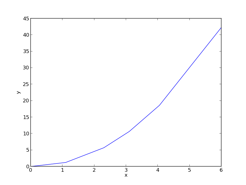
We are going to fit the function \(y = x^a\) to the data. The best \(a\) will minimize the summed squared error between the model and the fit.

def errfunc_(a):
    return np.sum((y - x**a)**2)

errfunc = np.vectorize(errfunc_)

arange = np.linspace(1, 3)
sse = errfunc(arange)

plt.figure()
plt.plot(arange, sse)
plt.xlabel('a')
plt.ylabel('$\Sigma (y - y_{pred})^2$')
plt.savefig('images/nonlin-minsse-2.png')
... >>> >>> >>> >>> >>> >>> <matplotlib.figure.Figure object at 0x000000000736DBA8>
[<matplotlib.lines.Line2D object at 0x00000000075CBEF0>]
<matplotlib.text.Text object at 0x00000000076B8C18>
<matplotlib.text.Text object at 0x0000000007698BE0>

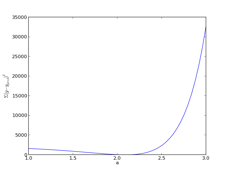
Based on the graph above, you can see a minimum in the summed squared error near \(a = 2.1\). We use that as our initial guess. Since we know the answer is bounded, we use scipy.optimize.fminbound

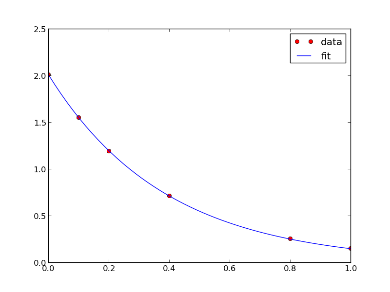
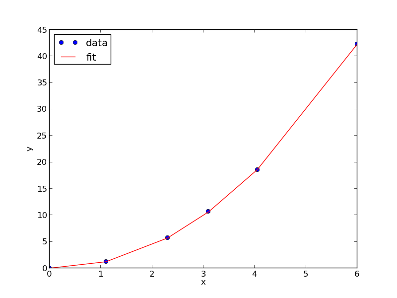
from scipy.optimize import fminbound

amin = fminbound(errfunc, 1.0, 3.0)

print amin

plt.figure()
plt.plot(x, y, 'bo', label='data')
plt.plot(x, x**amin, 'r-', label='fit')
plt.xlabel('x')
plt.ylabel('y')
plt.legend(loc='best')
plt.savefig('images/nonlin-minsse-3.png')
>>> >>> >>> 2.09004838933
>>> <matplotlib.figure.Figure object at 0x00000000075D8470>
[<matplotlib.lines.Line2D object at 0x0000000007BDFA20>]
[<matplotlib.lines.Line2D object at 0x0000000007BDFC18>]
<matplotlib.text.Text object at 0x0000000007BC6828>
<matplotlib.text.Text object at 0x0000000007BCAF98>
<matplotlib.legend.Legend object at 0x0000000007BE3128>

We can do nonlinear fitting by directly minimizing the summed squared error between a model and data. This method lacks some of the features of other methods, notably the simple ability to get the confidence interval. However, this method is flexible and may offer more insight into how the solution depends on the parameters.

Copyright (C) 2013 by John Kitchin. See the License for information about copying.

org-mode source

Discuss on Twitter

Fitting a numerical ODE solution to data

| categories: nonlinear regression, data analysis | tags:

Matlab post

Suppose we know the concentration of A follows this differential equation: \(\frac{dC_A}{dt} = -k C_A\), and we have data we want to fit to it. Here is an example of doing that.

import numpy as np
from scipy.optimize import curve_fit
from scipy.integrate import odeint

# given data we want to fit
tspan = [0, 0.1, 0.2, 0.4, 0.8, 1]
Ca_data = [2.0081,  1.5512,  1.1903,  0.7160,  0.2562,  0.1495]

def fitfunc(t, k):
    'Function that returns Ca computed from an ODE for a k'
    def myode(Ca, t):
        return -k * Ca

    Ca0 = Ca_data[0]
    Casol = odeint(myode, Ca0, t)
    return Casol[:,0]

k_fit, kcov = curve_fit(fitfunc, tspan, Ca_data, p0=1.3)
print k_fit

tfit = np.linspace(0,1);
fit = fitfunc(tfit, k_fit)

import matplotlib.pyplot as plt
plt.plot(tspan, Ca_data, 'ro', label='data')
plt.plot(tfit, fit, 'b-', label='fit')
plt.legend(loc='best')
plt.savefig('images/ode-fit.png')
[ 2.58893455]

Copyright (C) 2013 by John Kitchin. See the License for information about copying.

org-mode source

Discuss on Twitter

Are averages different

| categories: statistics, data analysis | tags:

Matlab post

Adapted from http://stattrek.com/ap-statistics-4/unpaired-means.aspx

Class A had 30 students who received an average test score of 78, with standard deviation of 10. Class B had 25 students an average test score of 85, with a standard deviation of 15. We want to know if the difference in these averages is statistically relevant. Note that we only have estimates of the true average and standard deviation for each class, and there is uncertainty in those estimates. As a result, we are unsure if the averages are really different. It could have just been luck that a few students in class B did better.

The hypothesis:

the true averages are the same. We need to perform a two-sample t-test of the hypothesis that \(\mu_1 - \mu_2 = 0\) (this is often called the null hypothesis). we use a two-tailed test because we do not care if the difference is positive or negative, either way means the averages are not the same.

import numpy as np

n1 = 30  # students in class A
x1 = 78.0  # average grade in class A
s1 = 10.0  # std dev of exam grade in class A

n2 = 25  # students in class B
x2 = 85.0  # average grade in class B
s2 = 15.0  # std dev of exam grade in class B

# the standard error of the difference between the two averages. 
SE = np.sqrt(s1**2 / n1 + s2**2 / n2)

# compute DOF
DF = (n1 - 1) + (n2 - 1)

see the discussion at http://stattrek.com/Help/Glossary.aspx?Target=Two-sample%20t-test for a more complex definition of degrees of freedom. Here we simply subtract one from each sample size to account for the estimation of the average of each sample.

compute the t-score for our data

The difference between two averages determined from small sample numbers follows the t-distribution. the t-score is the difference between the difference of the means and the hypothesized difference of the means, normalized by the standard error. we compute the absolute value of the t-score to make sure it is positive for convenience later.

tscore = np.abs(((x1 - x2) - 0) / SE)
print tscore
1.99323179108

Interpretation

A way to approach determinining if the difference is significant or not is to ask, does our computed average fall within a confidence range of the hypothesized value (zero)? If it does, then we can attribute the difference to statistical variations at that confidence level. If it does not, we can say that statistical variations do not account for the difference at that confidence level, and hence the averages must be different.

Let us compute the t-value that corresponds to a 95% confidence level for a mean of zero with the degrees of freedom computed earlier. This means that 95% of the t-scores we expect to get will fall within \(\pm\) t95.

from scipy.stats.distributions import  t

ci = 0.95;
alpha = 1 - ci;
t95 = t.ppf(1.0 - alpha/2.0, DF)

print t95
>>> >>> >>> >>> >>> 2.00574599354

since tscore < t95, we conclude that at the 95% confidence level we cannot say these averages are statistically different because our computed t-score falls in the expected range of deviations. Note that our t-score is very close to the 95% limit. Let us consider a smaller confidence interval.

ci = 0.94
alpha = 1 - ci;
t95 = t.ppf(1.0 - alpha/2.0, DF)

print t95
>>> >>> >>> 1.92191364181

at the 94% confidence level, however, tscore > t94, which means we can say with 94% confidence that the two averages are different; class B performed better than class A did. Alternatively, there is only about a 6% chance we are wrong about that statement. another way to get there

An alternative way to get the confidence that the averages are different is to directly compute it from the cumulative t-distribution function. We compute the difference between all the t-values less than tscore and the t-values less than -tscore, which is the fraction of measurements that are between them. You can see here that we are practically 95% sure that the averages are different.

f = t.cdf(tscore, DF) - t.cdf(-tscore, DF)
print f
0.948605075732

Copyright (C) 2013 by John Kitchin. See the License for information about copying.

org-mode source

Discuss on Twitter

Nonlinear curve fitting with confidence intervals

| categories: data analysis | tags:

Our goal is to fit this equation to data \(y = c1 exp(-x) + c2*x\) and compute the confidence intervals on the parameters.

This is actually could be a linear regression problem, but it is convenient to illustrate the use the nonlinear fitting routine because it makes it easy to get confidence intervals for comparison. The basic idea is to use the covariance matrix returned from the nonlinear fitting routine to estimate the student-t corrected confidence interval.

# Nonlinear curve fit with confidence interval
import numpy as np
from scipy.optimize import curve_fit
from scipy.stats.distributions import  t

x = np.array([ 0.1,  0.2,  0.3,  0.4,  0.5,  0.6,  0.7,  0.8,  0.9,  1. ])
y = np.array([ 4.70192769,  4.46826356,  4.57021389,  4.29240134,  3.88155125,
               3.78382253,  3.65454727,  3.86379487,  4.16428541,  4.06079909])

# this is the function we want to fit to our data
def func(x,c0, c1):
    return c0 * np.exp(-x) + c1*x

pars, pcov = curve_fit(func, x, y, p0=[4.96, 2.11])

alpha = 0.05 # 95% confidence interval

n = len(y)    # number of data points
p = len(pars) # number of parameters

dof = max(0, n-p) # number of degrees of freedom

tval = t.ppf(1.0 - alpha / 2.0, dof) # student-t value for the dof and confidence level

for i, p,var in zip(range(n), pars, np.diag(pcov)):
    sigma = var**0.5
    print 'c{0}: {1} [{2}  {3}]'.format(i, p,
                                  p - sigma*tval,
                                  p + sigma*tval)

import matplotlib.pyplot as plt
plt.plot(x,y,'bo ')
xfit = np.linspace(0,1)
yfit = func(xfit, pars[0], pars[1])
plt.plot(xfit,yfit,'b-')
plt.legend(['data','fit'],loc='best')
plt.savefig('images/nonlin-fit-ci.png')
c0: 4.96713966439 [4.62674476567  5.30753456311]
c1: 2.10995112628 [1.76711622427  2.45278602828]

Copyright (C) 2013 by John Kitchin. See the License for information about copying.

org-mode source

Discuss on Twitter

Nonlinear curve fitting

| categories: nonlinear regression, data analysis | tags:

Here is a typical nonlinear function fit to data. you need to provide an initial guess. In this example we fit the Birch-Murnaghan equation of state to energy vs. volume data from density functional theory calculations.

from scipy.optimize import leastsq
import numpy as np

vols = np.array([13.71, 14.82, 16.0, 17.23, 18.52])

energies = np.array([-56.29, -56.41, -56.46, -56.463, -56.41])

def Murnaghan(parameters, vol):
    'From Phys. Rev. B 28, 5480 (1983)'
    E0, B0, BP, V0 = parameters

    E = E0 + B0 * vol / BP * (((V0 / vol)**BP) / (BP - 1) + 1) - V0 * B0 / (BP - 1.0)

    return E

def objective(pars, y, x):
    #we will minimize this function
    err =  y - Murnaghan(pars, x)
    return err

x0 = [ -56.0, 0.54, 2.0, 16.5] #initial guess of parameters

plsq = leastsq(objective, x0, args=(energies, vols))

print 'Fitted parameters = {0}'.format(plsq[0])

import matplotlib.pyplot as plt
plt.plot(vols,energies, 'ro')

#plot the fitted curve on top
x = np.linspace(min(vols), max(vols), 50)
y = Murnaghan(plsq[0], x)
plt.plot(x, y, 'k-')
plt.xlabel('Volume')
plt.ylabel('Energy')
plt.savefig('images/nonlinear-curve-fitting.png')
Fitted parameters = [-56.46839641   0.57233217   2.7407944   16.55905648]

See additional examples at \url{http://docs.scipy.org/doc/scipy/reference/tutorial/optimize.html}.

Copyright (C) 2013 by John Kitchin. See the License for information about copying.

org-mode source

Discuss on Twitter
« Previous Page -- Next Page »