The Kitchin Research Group

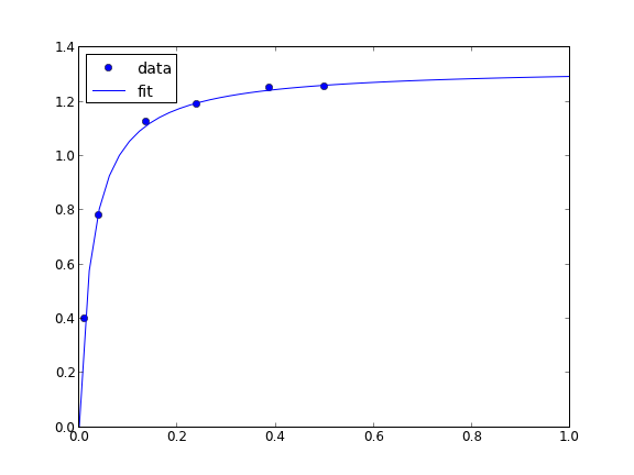
# Nonlinear curve fit with confidence interval
import numpy as np
from scipy.optimize import curve_fit
from scipy.stats.distributions import  t

x = np.array([ 0.1,  0.2,  0.3,  0.4,  0.5,  0.6,  0.7,  0.8,  0.9,  1. ])
y = np.array([ 4.70192769,  4.46826356,  4.57021389,  4.29240134,  3.88155125,
               3.78382253,  3.65454727,  3.86379487,  4.16428541,  4.06079909])

# this is the function we want to fit to our data
def func(x,c0, c1):
    return c0 * np.exp(-x) + c1*x

pars, pcov = curve_fit(func, x, y, p0=[4.96, 2.11])

alpha = 0.05 # 95% confidence interval

n = len(y)    # number of data points
p = len(pars) # number of parameters

dof = max(0, n-p) # number of degrees of freedom

tval = t.ppf(1.0 - alpha / 2.0, dof) # student-t value for the dof and confidence level

for i, p,var in zip(range(n), pars, np.diag(pcov)):
    sigma = var**0.5
    print 'c{0}: {1} [{2}  {3}]'.format(i, p,
                                  p - sigma*tval,
                                  p + sigma*tval)

import matplotlib.pyplot as plt
plt.plot(x,y,'bo ')
xfit = np.linspace(0,1)
yfit = func(xfit, pars[0], pars[1])
plt.plot(xfit,yfit,'b-')
plt.legend(['data','fit'],loc='best')
plt.savefig('images/nonlin-fit-ci.png')