Plane Poiseuille flow - BVP solve by shooting method

| categories: bvp | tags: fluids

Matlab post

One approach to solving BVPs is to use the shooting method. The reason we cannot use an initial value solver for a BVP is that there is not enough information at the initial value to start. In the shooting method, we take the function value at the initial point, and guess what the function derivatives are so that we can do an integration. If our guess was good, then the solution will go through the known second boundary point. If not, we guess again, until we get the answer we need. In this example we repeat the pressure driven flow example, but illustrate the shooting method.

In the pressure driven flow of a fluid with viscosity \(\mu\) between two stationary plates separated by distance \(d\) and driven by a pressure drop \(\Delta P/\Delta x\), the governing equations on the velocity \(u\) of the fluid are (assuming flow in the x-direction with the velocity varying only in the y-direction):

$$\frac{\Delta P}{\Delta x} = \mu \frac{d^2u}{dy^2}$$

with boundary conditions \(u(y=0) = 0\) and \(u(y=d) = 0\), i.e. the no-slip condition at the edges of the plate.

we convert this second order BVP to a system of ODEs by letting \(u_1 = u\), \(u_2 = u_1'\) and then \(u_2' = u_1''\). This leads to:

\(\frac{d u_1}{dy} = u_2\)

\(\frac{d u_2}{dy} = \frac{1}{\mu}\frac{\Delta P}{\Delta x}\)

with boundary conditions \(u_1(y=0) = 0\) and \(u_1(y=d) = 0\).

for this problem we let the plate separation be d=0.1, the viscosity \(\mu = 1\), and \(\frac{\Delta P}{\Delta x} = -100\).

1 First guess

We need u_1(0) and u_2(0), but we only have u_1(0). We need to guess a value for u_2(0) and see if the solution goes through the u_2(d)=0 boundary value.

import numpy as np
from scipy.integrate import odeint
import matplotlib.pyplot as plt

d = 0.1 # plate thickness

def odefun(U, y):
    u1, u2 = U
    mu = 1
    Pdrop = -100
    du1dy = u2
    du2dy = 1.0 / mu * Pdrop
    return [du1dy, du2dy]

u1_0 = 0 # known
u2_0 = 1 # guessed

dspan = np.linspace(0, d)

U = odeint(odefun, [u1_0, u2_0], dspan)

plt.plot(dspan, U[:,0])
plt.plot([d],[0], 'ro')
plt.xlabel('d')
plt.ylabel('$u_1$')
plt.savefig('images/bvp-shooting-1.png')

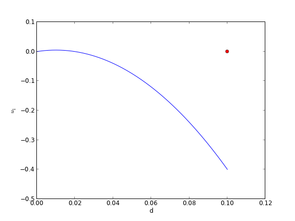
Here we have undershot the boundary condition. Let us try a larger guess.

2 Second guess

import numpy as np
from scipy.integrate import odeint
import matplotlib.pyplot as plt

d = 0.1 # plate thickness

def odefun(U, y):
    u1, u2 = U
    mu = 1
    Pdrop = -100
    du1dy = u2
    du2dy = 1.0 / mu * Pdrop
    return [du1dy, du2dy]

u1_0 = 0 # known
u2_0 = 10 # guessed

dspan = np.linspace(0, d)

U = odeint(odefun, [u1_0, u2_0], dspan)

plt.plot(dspan, U[:,0])
plt.plot([d],[0], 'ro')
plt.xlabel('d')
plt.ylabel('$u_1$')
plt.savefig('images/bvp-shooting-2.png')

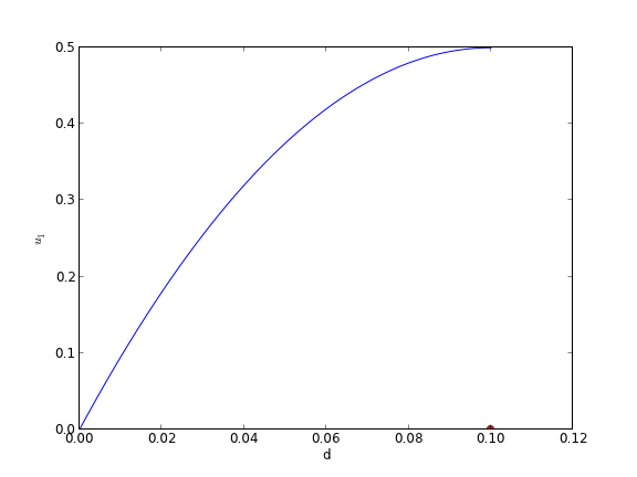
Now we have clearly overshot. Let us now make a function that will iterate for us to find the right value.

3 Let fsolve do the work

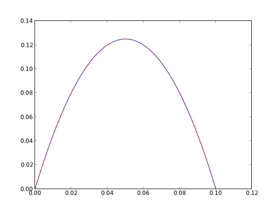
import numpy as np
from scipy.integrate import odeint
from scipy.optimize import fsolve
import matplotlib.pyplot as plt

d = 0.1 # plate thickness
Pdrop = -100
mu = 1

def odefun(U, y):
    u1, u2 = U
    du1dy = u2
    du2dy = 1.0 / mu * Pdrop
    return [du1dy, du2dy]

u1_0 = 0 # known
dspan = np.linspace(0, d)

def objective(u2_0):
    dspan = np.linspace(0, d)
    U = odeint(odefun, [u1_0, u2_0], dspan)
    u1 = U[:,0]
    return u1[-1]

u2_0, = fsolve(objective, 1.0)

# now solve with optimal u2_0
U = odeint(odefun, [u1_0, u2_0], dspan)

plt.plot(dspan, U[:,0], label='Numerical solution')
plt.plot([d],[0], 'ro')

# plot an analytical solution
u = -(Pdrop) * d**2 / 2 / mu * (dspan / d - (dspan / d)**2)
plt.plot(dspan, u, 'r--', label='Analytical solution')


plt.xlabel('d')
plt.ylabel('$u_1$')
plt.legend(loc='best')
plt.savefig('images/bvp-shooting-3.png')

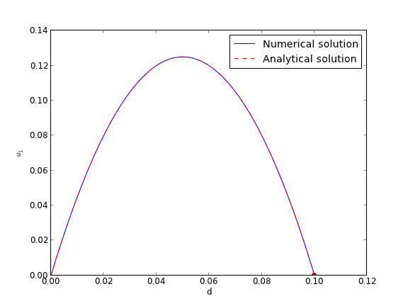
You can see the agreement is excellent!

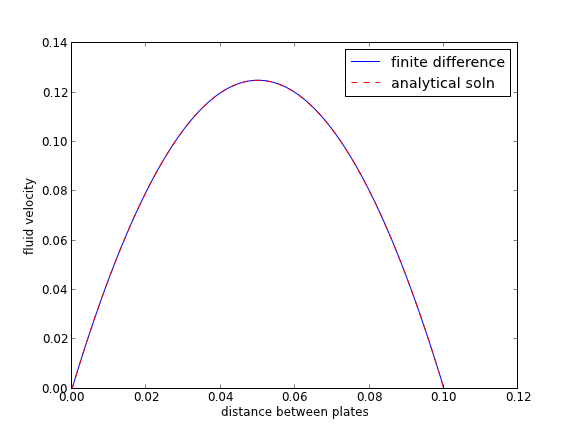
This also seems like a useful bit of code to not have to reinvent regularly, so it has been added to pycse as BVP_sh. Here is an example usage.

from pycse import BVP_sh
import matplotlib.pyplot as plt

d = 0.1 # plate thickness
Pdrop = -100
mu = 1

def odefun(U, y):
    u1, u2 = U
    du1dy = u2
    du2dy = 1.0 / mu * Pdrop
    return [du1dy, du2dy]

x1 = 0.0; alpha = 0.0
x2 = 0.1; beta = 0.0
init = 2.0 # initial guess of slope at x=0

X,Y = BVP_sh(odefun, x1, x2, alpha, beta, init)
plt.plot(X, Y[:,0])
plt.ylim([0, 0.14])

# plot an analytical solution
u = -(Pdrop) * d**2 / 2 / mu * (X / d - (X / d)**2)
plt.plot(X, u, 'r--', label='Analytical solution')
plt.savefig('images/bvp-shooting-4.png')
plt.show()

Copyright (C) 2013 by John Kitchin. See the License for information about copying.

org-mode source

Discuss on Twitter

Plane poiseuelle flow solved by finite difference

| categories: bvp | tags: fluids

Matlab post

Adapted from http://www.physics.arizona.edu/~restrepo/475B/Notes/sourcehtml/node24.html

We want to solve a linear boundary value problem of the form: y'' = p(x)y' + q(x)y + r(x) with boundary conditions y(x1) = alpha and y(x2) = beta.

For this example, we solve the plane poiseuille flow problem using a finite difference approach. An advantage of the approach we use here is we do not have to rewrite the second order ODE as a set of coupled first order ODEs, nor do we have to provide guesses for the solution. We do, however, have to discretize the derivatives and formulate a linear algebra problem.

we want to solve u'' = 1/mu*DPDX with u(0)=0 and u(0.1)=0. for this problem we let the plate separation be d=0.1, the viscosity \(\mu = 1\), and \(\frac{\Delta P}{\Delta x} = -100\).

The idea behind the finite difference method is to approximate the derivatives by finite differences on a grid. See here for details. By discretizing the ODE, we arrive at a set of linear algebra equations of the form \(A y = b\), where \(A\) and \(b\) are defined as follows.

\[A = \left [ \begin{array}{ccccc} % 2 + h^2 q_1 & -1 + \frac{h}{2} p_1 & 0 & 0 & 0 \\ -1 - \frac{h}{2} p_2 & 2 + h^2 q_2 & -1 + \frac{h}{2} p_2 & 0 & 0 \\ 0 & \ddots & \ddots & \ddots & 0 \\ 0 & 0 & -1 - \frac{h}{2} p_{N-1} & 2 + h^2 q_{N-1} & -1 + \frac{h}{2} p_{N-1} \\ 0 & 0 & 0 & -1 - \frac{h}{2} p_N & 2 + h^2 q_N \end{array} \right ] \]

\[ y = \left [ \begin{array}{c} y_i \\ \vdots \\ y_N \end{array} \right ] \]

\[ b = \left [ \begin{array}{c} -h^2 r_1 + ( 1 + \frac{h}{2} p_1) \alpha \\ -h^2 r_2 \\ \vdots \\ -h^2 r_{N-1} \\ -h^2 r_N + (1 - \frac{h}{2} p_N) \beta \end{array} \right] \]

import numpy as np

# we use the notation for y'' = p(x)y' + q(x)y + r(x)
def p(x): return 0
def q(x): return 0
def r(x): return -100

#we use the notation y(x1) = alpha and y(x2) = beta

x1 = 0; alpha = 0.0
x2 = 0.1; beta = 0.0

npoints = 100

# compute interval width
h = (x2-x1)/npoints;

# preallocate and shape the b vector and A-matrix
b = np.zeros((npoints - 1, 1));
A = np.zeros((npoints - 1, npoints - 1));
X = np.zeros((npoints - 1, 1));

#now we populate the A-matrix and b vector elements
for i in range(npoints - 1):
    X[i,0] = x1 + (i + 1) * h

    # get the value of the BVP Odes at this x
    pi = p(X[i])
    qi = q(X[i])
    ri = r(X[i])

    if i == 0:
        # first boundary condition
        b[i] = -h**2 * ri + (1 + h / 2 * pi)*alpha; 
    elif i == npoints - 1:
        # second boundary condition
        b[i] = -h**2 * ri + (1 - h / 2 * pi)*beta; 
    else:
        b[i] = -h**2 * ri # intermediate points
    
    for j in range(npoints - 1):
        if j == i: # the diagonal
            A[i,j] = 2 + h**2 * qi
        elif j == i - 1: # left of the diagonal
            A[i,j] = -1 - h / 2 * pi
        elif j == i + 1: # right of the diagonal
            A[i,j] = -1 + h / 2 * pi
        else:
            A[i,j] = 0 # off the tri-diagonal
 
# solve the equations A*y = b for Y
Y = np.linalg.solve(A,b)

x = np.hstack([x1, X[:,0], x2])
y = np.hstack([alpha, Y[:,0], beta])

import matplotlib.pyplot as plt

plt.plot(x, y)

mu = 1
d = 0.1
x = np.linspace(0,0.1);
Pdrop = -100 # this is DeltaP/Deltax
u = -(Pdrop) * d**2 / 2.0 / mu * (x / d - (x / d)**2)
plt.plot(x,u,'r--')

plt.xlabel('distance between plates')
plt.ylabel('fluid velocity')
plt.legend(('finite difference', 'analytical soln'))
plt.savefig('images/pp-bvp-fd.png')
plt.show()

You can see excellent agreement here between the numerical and analytical solution.

Copyright (C) 2013 by John Kitchin. See the License for information about copying.

org-mode source

Discuss on Twitter

Numerically calculating an effectiveness factor for a porous catalyst bead

| categories: bvp | tags: reaction engineering

Matlab post

If reaction rates are fast compared to diffusion in a porous catalyst pellet, then the observed kinetics will appear to be slower than they really are because not all of the catalyst surface area will be effectively used. For example, the reactants may all be consumed in the near surface area of a catalyst bead, and the inside of the bead will be unutilized because no reactants can get in due to the high reaction rates.

References: Ch 12. Elements of Chemical Reaction Engineering, Fogler, 4th edition.

A mole balance on the particle volume in spherical coordinates with a first order reaction leads to: $\frac{d^2Ca}{dr^2} + \frac{2}{r}\frac{dCa}{dr}-\frac{k}{D_e}C_A=0$ with boundary conditions $C_A(R) = C_{As}$ and $\frac{dCa}{dr}=0$ at $r=0$. We convert this equation to a system of first order ODEs by letting $W_A=\frac{dCa}{dr}$. Then, our two equations become:

\(\frac{dCa}{dr} = W_A\)

and

\(\frac{dW_A}{dr} = -\frac{2}{r} W_A + \frac{k}{D_E} C_A\)

We have a condition of no flux ($W_A=0$
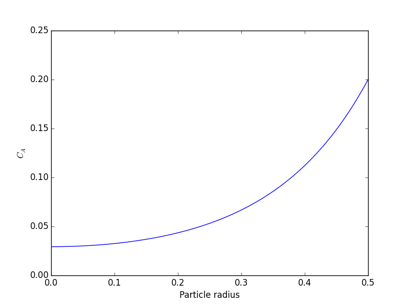
) at r=0 and Ca(R) = CAs, which makes this a boundary value problem. We use the shooting method here, and guess what Ca(0) is and iterate the guess to get Ca(R) = CAs.

The value of the second differential equation at r=0 is tricky because at this place we have a 0/0 term. We use L'Hopital's rule to evaluate it. The derivative of the top is $\frac{dW_A}{dr}$ and the derivative of the bottom is 1. So, we have \(\frac{dW_A}{dr} = -2\frac{dW_A}{dr} + \frac{k}{D_E} C_A\)

Which leads to:

\(3 \frac{dW_A}{dr} =  \frac{k}{D_E} C_A\)

or \(\frac{dW_A}{dr} =  \frac{3k}{D_E} C_A\) at $r=0$.

Finally, we implement the equations in Python and solve.

import numpy as np
from scipy.integrate import odeint
import matplotlib.pyplot as plt

De = 0.1    # diffusivity cm^2/s
R = 0.5    # particle radius, cm
k = 6.4    # rate constant (1/s)
CAs = 0.2   # concentration of A at outer radius of particle (mol/L)


def ode(Y, r):
    Wa = Y[0]  # molar rate of delivery of A to surface of particle
    Ca = Y[1]  # concentration of A in the particle at r
    # this solves the singularity at r = 0
    if r == 0:
        dWadr = k / 3.0 * De * Ca
    else:
        dWadr = -2 * Wa / r + k / De * Ca
    dCadr = Wa
    return [dWadr, dCadr]

# Initial conditions
Ca0 = 0.029315  # Ca(0) (mol/L) guessed to satisfy Ca(R) = CAs
Wa0 = 0         # no flux at r=0 (mol/m^2/s)

rspan = np.linspace(0, R, 500)

Y = odeint(ode, [Wa0, Ca0], rspan)

Ca = Y[:, 1]

# here we check that Ca(R) = Cas
print 'At r={0} Ca={1}'.format(rspan[-1], Ca[-1])

plt.plot(rspan, Ca)
plt.xlabel('Particle radius')
plt.ylabel('$C_A$')
plt.savefig('images/effectiveness-factor.png')

r = rspan
eta_numerical = (np.trapz(k * Ca * 4 * np.pi * (r**2), r)
                 / np.trapz(k * CAs * 4 * np.pi * (r**2), r))

print(eta_numerical)

phi = R * np.sqrt(k / De)
eta_analytical = (3 / phi**2) * (phi * (1.0 / np.tanh(phi)) - 1)
print(eta_analytical)
At r=0.5 Ca=0.200001488652
[<matplotlib.lines.Line2D object at 0x114275550>]
<matplotlib.text.Text object at 0x10d5fe890>
<matplotlib.text.Text object at 0x10d5ff890>
0.563011348314

0.563003362801

You can see the concentration of A inside the particle is significantly lower than outside the particle. That is because it is reacting away faster than it can diffuse into the particle. Hence, the overall reaction rate in the particle is lower than it would be without the diffusion limit.

The effectiveness factor is the ratio of the actual reaction rate in the particle with diffusion limitation to the ideal rate in the particle if there was no concentration gradient:

$$\eta = \frac{\int_0^R k'' a C_A(r) 4 \pi r^2 dr}{\int_0^R k'' a C_{As} 4 \pi r^2 dr}$$

We will evaluate this numerically from our solution and compare it to the analytical solution. The results are in good agreement, and you can make the numerical estimate better by increasing the number of points in the solution so that the numerical integration is more accurate.

Why go through the numerical solution when an analytical solution exists? The analytical solution here is only good for 1st order kinetics in a sphere. What would you do for a complicated rate law? You might be able to find some limiting conditions where the analytical equation above is relevant, and if you are lucky, they are appropriate for your problem. If not, it is a good thing you can figure this out numerically!

Thanks to Radovan Omorjan for helping me figure out the ODE at r=0!

Copyright (C) 2015 by John Kitchin. See the License for information about copying.

org-mode source

Org-mode version = 8.2.10

Discuss on Twitter
« Previous Page