The Kitchin Research Group

Matlab post

Adapted from http://www.physics.arizona.edu/~restrepo/475B/Notes/sourcehtml/node24.html

We want to solve a linear boundary value problem of the form: y'' = p(x)y' + q(x)y + r(x) with boundary conditions y(x1) = alpha and y(x2) = beta.

For this example, we solve the plane poiseuille flow problem using a finite difference approach. An advantage of the approach we use here is we do not have to rewrite the second order ODE as a set of coupled first order ODEs, nor do we have to provide guesses for the solution. We do, however, have to discretize the derivatives and formulate a linear algebra problem.

we want to solve u'' = 1/mu*DPDX with u(0)=0 and u(0.1)=0. for this problem we let the plate separation be d=0.1, the viscosity \(\mu = 1\), and \(\frac{\Delta P}{\Delta x} = -100\).

The idea behind the finite difference method is to approximate the derivatives by finite differences on a grid. See here for details. By discretizing the ODE, we arrive at a set of linear algebra equations of the form \(A y = b\), where \(A\) and \(b\) are defined as follows.

\[A = \left [ \begin{array}{ccccc} % 2 + h^2 q_1 & -1 + \frac{h}{2} p_1 & 0 & 0 & 0 \\ -1 - \frac{h}{2} p_2 & 2 + h^2 q_2 & -1 + \frac{h}{2} p_2 & 0 & 0 \\ 0 & \ddots & \ddots & \ddots & 0 \\ 0 & 0 & -1 - \frac{h}{2} p_{N-1} & 2 + h^2 q_{N-1} & -1 + \frac{h}{2} p_{N-1} \\ 0 & 0 & 0 & -1 - \frac{h}{2} p_N & 2 + h^2 q_N \end{array} \right ] \]

\[ y = \left [ \begin{array}{c} y_i \\ \vdots \\ y_N \end{array} \right ] \]

\[ b = \left [ \begin{array}{c} -h^2 r_1 + ( 1 + \frac{h}{2} p_1) \alpha \\ -h^2 r_2 \\ \vdots \\ -h^2 r_{N-1} \\ -h^2 r_N + (1 - \frac{h}{2} p_N) \beta \end{array} \right] \]

import numpy as np

# we use the notation for y'' = p(x)y' + q(x)y + r(x)
def p(x): return 0
def q(x): return 0
def r(x): return -100

#we use the notation y(x1) = alpha and y(x2) = beta

x1 = 0; alpha = 0.0
x2 = 0.1; beta = 0.0

npoints = 100

# compute interval width
h = (x2-x1)/npoints;

# preallocate and shape the b vector and A-matrix
b = np.zeros((npoints - 1, 1));
A = np.zeros((npoints - 1, npoints - 1));
X = np.zeros((npoints - 1, 1));

#now we populate the A-matrix and b vector elements
for i in range(npoints - 1):
    X[i,0] = x1 + (i + 1) * h

    # get the value of the BVP Odes at this x
    pi = p(X[i])
    qi = q(X[i])
    ri = r(X[i])

    if i == 0:
        # first boundary condition
        b[i] = -h**2 * ri + (1 + h / 2 * pi)*alpha; 
    elif i == npoints - 1:
        # second boundary condition
        b[i] = -h**2 * ri + (1 - h / 2 * pi)*beta; 
    else:
        b[i] = -h**2 * ri # intermediate points
    
    for j in range(npoints - 1):
        if j == i: # the diagonal
            A[i,j] = 2 + h**2 * qi
        elif j == i - 1: # left of the diagonal
            A[i,j] = -1 - h / 2 * pi
        elif j == i + 1: # right of the diagonal
            A[i,j] = -1 + h / 2 * pi
        else:
            A[i,j] = 0 # off the tri-diagonal
 
# solve the equations A*y = b for Y
Y = np.linalg.solve(A,b)

x = np.hstack([x1, X[:,0], x2])
y = np.hstack([alpha, Y[:,0], beta])

import matplotlib.pyplot as plt

plt.plot(x, y)

mu = 1
d = 0.1
x = np.linspace(0,0.1);
Pdrop = -100 # this is DeltaP/Deltax
u = -(Pdrop) * d**2 / 2.0 / mu * (x / d - (x / d)**2)
plt.plot(x,u,'r--')

plt.xlabel('distance between plates')
plt.ylabel('fluid velocity')
plt.legend(('finite difference', 'analytical soln'))
plt.savefig('images/pp-bvp-fd.png')
plt.show()

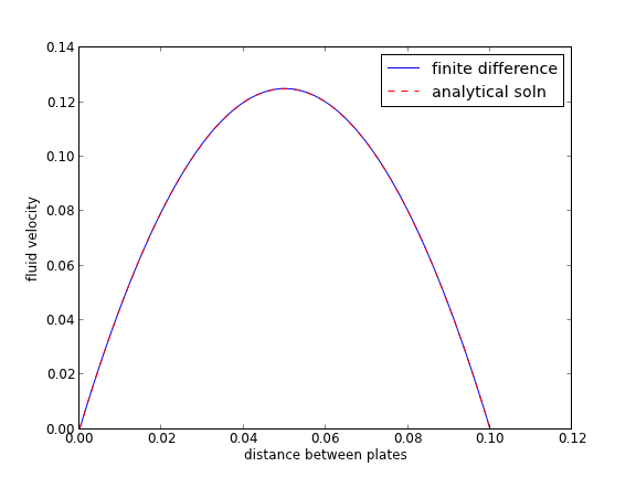
You can see excellent agreement here between the numerical and analytical solution.

Copyright (C) 2013 by John Kitchin. See the License for information about copying.

org-mode source