Solving an eigenvalue differential equation with a neural network

| categories: autograd, bvp, eigenvalue | tags:

The 1D harmonic oscillator is described here. It is a boundary value differential equation with eigenvalues. If we let let ω=1, m=1, and units where ℏ=1. then, the governing differential equation becomes:

\(-0.5 \frac{d^2\psi(x)}{dx^2} + (0.5 x^2 - E) \psi(x) = 0\)

with boundary conditions: \(\psi(-\infty) = \psi(\infty) = 0\)

We can further stipulate that the probability of finding the particle over this domain is equal to one: \(\int_{-\infty}^{\infty} \psi^2(x) dx = 1\). In this set of equations, \(E\) is an eigenvalue, which means there are only non-trivial solutions for certain values of \(E\).

Our goal is to solve this equation using a neural network to represent the wave function. This is a different problem than the one here or here because of the eigenvalue. This is an additional adjustable parameter we have to find. Also, we have the normalization constraint to consider, which we did not consider before.

1 The neural network setup

Here we setup the neural network and its derivatives. This is the same as we did before.

import autograd.numpy as np
from autograd import grad, elementwise_grad
import autograd.numpy.random as npr
from autograd.misc.optimizers import adam

def init_random_params(scale, layer_sizes, rs=npr.RandomState(42)):
    """Build a list of (weights, biases) tuples, one for each layer."""
    return [(rs.randn(insize, outsize) * scale,   # weight matrix
             rs.randn(outsize) * scale)           # bias vector
            for insize, outsize in zip(layer_sizes[:-1], layer_sizes[1:])]

def swish(x):
    "see https://arxiv.org/pdf/1710.05941.pdf"
    return x / (1.0 + np.exp(-x))

def psi(nnparams, inputs):
    "Neural network wavefunction"
    for W, b in nnparams:
        outputs = np.dot(inputs, W) + b
        inputs = swish(outputs)    
    return outputs

psip = elementwise_grad(psi, 1) # dpsi/dx 
psipp = elementwise_grad(psip, 1) # d^2psi/dx^2

2 The objective function

The important function we need is the objective function. This function codes the Schrödinger equation, the boundary conditions, and the normalization as a cost function that we will later seek to minimize. Ideally, at the solution the objective function will be zero. We can't put infinity into our objective function, but it turns out that x = ± 6 is practically infinity in this case, so we approximate the boundary conditions there.

Another note is the numerical integration by the trapezoid rule. I use a vectorized version of this because autograd doesn't have a trapz derivative and I didn't feel like figuring one out.

We define the params to vary here as a dictionary containing neural network weights and biases, and the value of the eigenvalue.

# Here is our initial guess of params:
nnparams = init_random_params(0.1, layer_sizes=[1, 8, 1])

params = {'nn': nnparams, 'E': 0.4}

x = np.linspace(-6, 6, 200)[:, None]

def objective(params, step):
    nnparams = params['nn']
    E = params['E']        
    # This is Schrodinger's eqn
    zeq = -0.5 * psipp(nnparams, x) + (0.5 * x**2 - E) * psi(nnparams, x) 
    bc0 = psi(nnparams, -6.0) # This approximates -infinity
    bc1 = psi(nnparams, 6.0)  # This approximates +infinity
    y2 = psi(nnparams, x)**2
    # This is a numerical trapezoid integration
    prob = np.sum((y2[1:] + y2[0:-1]) / 2 * (x[1:] - x[0:-1]))
    return np.mean(zeq**2) + bc0**2 + bc1**2 + (1.0 - prob)**2

# This gives us feedback from the optimizer
def callback(params, step, g):
    if step % 1000 == 0:
        print("Iteration {0:3d} objective {1}".format(step,
                                                      objective(params, step)))

3 The minimization

Now, we just let an optimizer minimize the objective function for us. Note, I ran this next block more than once, as the objective continued to decrease. I ran this one at least two times, and the loss was still decreasing slowly.

params = adam(grad(objective), params,
              step_size=0.001, num_iters=5001, callback=callback) 

print(params['E'])
Iteration   0 objective [[ 0.00330204]]
Iteration 1000 objective [[ 0.00246459]]
Iteration 2000 objective [[ 0.00169862]]
Iteration 3000 objective [[ 0.00131453]]
Iteration 4000 objective [[ 0.00113132]]
Iteration 5000 objective [[ 0.00104405]]
0.5029457355415167

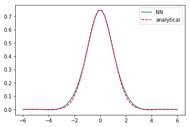
Good news, the lowest energy eigenvalue is known to be 0.5 for our choice of parameters, and that is approximately what we got. Now let's see our solution and compare it to the known solution. Interestingly we got the negative of the solution, which is still a solution. The NN solution is not indistinguishable from the analytical solution, and has some spurious curvature in the tails, but it is approximately correct, and more training might get it closer. A different activation function might also work better.

%matplotlib inline
import matplotlib.pyplot as plt

x = np.linspace(-6, 6)[:, None]
y = psi(params['nn'], x)

plt.plot(x, -y, label='NN')
plt.plot(x, (1/np.pi)**0.25 * np.exp(-x**2 / 2), 'r--', label='analytical')
plt.legend()

4 The first excited state

Now, what about the first excited state? This has an eigenvalue of 1.5, and the solution has odd parity. We can naively change the eigenvalue, and hope that the optimizer will find the right new solution. We do that here, and use the old NN params.

params['E'] = 1.6

Now, we run a round of optimization:

params = adam(grad(objective), params,
              step_size=0.003, num_iters=5001, callback=callback) 

print(params['E'])
Iteration   0 objective [[ 0.09918192]]
Iteration 1000 objective [[ 0.00102333]]
Iteration 2000 objective [[ 0.00100269]]
Iteration 3000 objective [[ 0.00098684]]
Iteration 4000 objective [[ 0.00097425]]
Iteration 5000 objective [[ 0.00096347]]
0.502326347406645

That doesn't work though. The optimizer just pushes the solution back to the known one. Next, we try starting from scratch with the eigenvalue guess.

nnparams = init_random_params(0.1, layer_sizes=[1, 8, 1])

params = {'nn': nnparams, 'E': 1.6}

params = adam(grad(objective), params,
              step_size=0.003, num_iters=5001, callback=callback) 

print(params['E'])
Iteration   0 objective [[ 2.08318762]]
Iteration 1000 objective [[ 0.02358685]]
Iteration 2000 objective [[ 0.00726497]]
Iteration 3000 objective [[ 0.00336433]]
Iteration 4000 objective [[ 0.00229851]]
Iteration 5000 objective [[ 0.00190942]]
0.5066213334684926

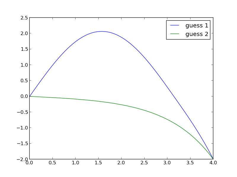
That also doesn't work. We are going to have to steer this. The idea is pre-train the neural network to have the basic shape and symmetry we want, and then use that as the input for the objective function. The first excited state has odd parity, and here is a guess of that shape. This is a pretty ugly hacked up version that only roughly has the right shape. I am counting on the NN smoothing out the discontinuities.

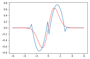
xm = np.linspace(-6, 6)[:, None]
ym = -0.5 * ((-1 * (xm + 1.5)**2) + 1.5) * (xm < 0) * (xm > -3)
yp = -0.5 * ((1 * (xm - 1.5)**2 ) - 1.5) * (xm > 0) * (xm < 3)

plt.plot(xm, (ym + yp))
plt.plot(x, (1/np.pi)**0.25 * np.sqrt(2) * x * np.exp(-x**2 / 2), 'r--', label='analytical')

Now we pretrain a bit.

def pretrain(params, step):
    nnparams = params['nn']
    errs = psi(nnparams, xm) - (ym + yp)
    return np.mean(errs**2)

params = adam(grad(pretrain), params,
              step_size=0.003, num_iters=501, callback=callback) 
Iteration   0 objective [[ 1.09283695]]

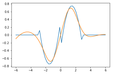
Here is the new initial guess we are going to use. You can see that indeed a lot of smoothing has occurred.

plt.plot(xm, ym + yp, xm, psi(params['nn'], xm))

That has the right shape now. So we go back to the original objective function.

params = adam(grad(objective), params,
              step_size=0.001, num_iters=5001, callback=callback) 

print(params['E'])
Iteration   0 objective [[ 0.00370029]]
Iteration 1000 objective [[ 0.00358193]]
Iteration 2000 objective [[ 0.00345137]]
Iteration 3000 objective [[ 0.00333]]
Iteration 4000 objective [[ 0.0032198]]
Iteration 5000 objective [[ 0.00311844]]
1.5065724128094344

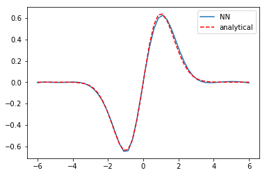
I ran that optimization block many times. The loss is still decreasing, but slowly. More importantly, the eigenvalue is converging to 1.5, which is the known analytical value, and the solution is converging to the known solution.

x = np.linspace(-6, 6)[:, None]
y = psi(params['nn'], x)

plt.plot(x, y, label='NN')
plt.plot(x, (1/np.pi)**0.25 * np.sqrt(2) * x * np.exp(-x**2 / 2), 'r--', label='analytical')
plt.legend()

We can confirm the normalization is reasonable:

# check the normalization
print(np.trapz(y.T * y.T, x.T))
[ 0.99781886]

5 Summary

This is another example of using autograd to solve an eigenvalue differential equation. Some of these solutions required tens of thousands of iterations of training. The groundstate wavefunction was very easy to get. The first excited state, on the other hand, took some active steering. This is very much like how an initial guess can change which solution a nonlinear optimization (which this is) finds.

There are other ways to solve this particular problem. What I think is interesting about this is the possibility to solve harder problems, e.g. not just a harmonic potential, but a more complex one. You could pretrain a network on the harmonic solution, and then use it as the initial guess for the harder problem (which has no analytical solution).

Copyright (C) 2017 by John Kitchin. See the License for information about copying.

org-mode source

Org-mode version = 9.1.2

Discuss on Twitter

Solving BVPs with a neural network and autograd

| categories: autograd, bvp | tags:

In this post we solved a boundary value problem by discretizing it, and approximating the derivatives by finite differences. Here I explore using a neural network to approximate the unknown function, autograd to get the required derivatives, and using autograd to train the neural network to satisfy the differential equations. We will look at the Blasius equation again.

\begin{eqnarray} f''' + \frac{1}{2} f f'' &=& 0 \\ f(0) &=& 0 \\ f'(0) &=& 0 \\ f'(\infty) &=& 1 \end{eqnarray}

Here I setup a simple neural network

import autograd.numpy as np
from autograd import grad, elementwise_grad
import autograd.numpy.random as npr
from autograd.misc.optimizers import adam

def init_random_params(scale, layer_sizes, rs=npr.RandomState(0)):
    """Build a list of (weights, biases) tuples, one for each layer."""
    return [(rs.randn(insize, outsize) * scale,   # weight matrix
             rs.randn(outsize) * scale)           # bias vector
            for insize, outsize in zip(layer_sizes[:-1], layer_sizes[1:])]


def swish(x):
    "see https://arxiv.org/pdf/1710.05941.pdf"
    return x / (1.0 + np.exp(-x))


def f(params, inputs):
    "Neural network functions"
    for W, b in params:
        outputs = np.dot(inputs, W) + b
        inputs = swish(outputs)    
    return outputs

    
# Here is our initial guess of params:
params = init_random_params(0.1, layer_sizes=[1, 8, 1])

# Derivatives
fp = elementwise_grad(f, 1)
fpp = elementwise_grad(fp, 1)
fppp = elementwise_grad(fpp, 1)

eta = np.linspace(0, 6).reshape((-1, 1))

# This is the function we seek to minimize
def objective(params, step):
    # These should all be zero at the solution
    # f''' + 0.5 f'' f = 0
    zeq = fppp(params, eta) + 0.5 * f(params, eta) * fpp(params, eta) 
    bc0 = f(params, 0.0)  # equal to zero at solution
    bc1 = fp(params, 0.0)  # equal to zero at solution
    bc2 = fp(params, 6.0) - 1.0 # this is the one at "infinity"
    return np.mean(zeq**2) + bc0**2 + bc1**2 + bc2**2

def callback(params, step, g):
    if step % 1000 == 0:
        print("Iteration {0:3d} objective {1}".format(step,
                                                      objective(params, step)))

params = adam(grad(objective), params,
              step_size=0.001, num_iters=10000, callback=callback) 

print('f(0) = {}'.format(f(params, 0.0)))
print('fp(0) = {}'.format(fp(params, 0.0)))
print('fp(6) = {}'.format(fp(params, 6.0)))
print('fpp(0) = {}'.format(fpp(params, 0.0)))

import matplotlib.pyplot as plt
plt.plot(eta, f(params, eta))
plt.xlabel('$\eta$')
plt.ylabel('$f(\eta)$')
plt.xlim([0, 6])
plt.ylim([0, 4.5])
plt.savefig('nn-blasius.png')

Iteration 0 objective 1.11472535 Iteration 1000 objective 0.00049768 Iteration 2000 objective 0.0004579 Iteration 3000 objective 0.00041697 Iteration 4000 objective 0.00037408 Iteration 5000 objective 0.00033705 Iteration 6000 objective 0.00031016 Iteration 7000 objective 0.00029197 Iteration 8000 objective 0.00027585 Iteration 9000 objective 0.00024616 f(0) = -0.00014613 fp(0) = 0.0003518041251639459 fp(6) = 0.999518061473252 fpp(0) = 0.3263370503702663

I think it is worth discussing what we accomplished here. You can see we have arrived at an approximate solution to our differential equation and the boundary conditions. The boundary conditions seem pretty closely met, and the figure is approximately the same as the previous post. Even better, our solution is an actual function and not a numeric solution that has to be interpolated. We can evaluate it any where we want, including its derivatives!

We did not, however, have to convert the ODE into a system of first-order differential equations, and we did not have to approximate the derivatives with finite differences.

Note, however, that with finite differences we got f''(0)=0.3325. This site reports f''(0)=0.3321. We get close to that here with f''(0) = 0.3263. We could probably get closer to this with more training to reduce the objective function further, or with a finer grid. It is evident that even after 9000 steps, it is still decreasing. Getting accurate derivatives is a stringent test for this, as they are measures of the function curvature.

It is hard to tell how broadly useful this is; I have not tried it beyond this example. In the past, I have found solving BVPs to be pretty sensitive to the initial guesses of the solution. Here we made almost no guess at all, and still got a solution. I find that pretty remarkable.

Copyright (C) 2017 by John Kitchin. See the License for information about copying.

org-mode source

Org-mode version = 9.1.2

Discuss on Twitter

Solving the Blasius equation

| categories: bvp | tags:

In fluid mechanics the Blasius equation comes up (http://en.wikipedia.org/wiki/Blasius_boundary_layer) to describe the boundary layer that forms near a flat plate with fluid moving by it. The nonlinear differential equation is:

\begin{eqnarray} f''' + \frac{1}{2} f f'' &=& 0 \\ f(0) &=& 0 \\ f'(0) &=& 0 \\ f'(\infty) &=& 1 \end{eqnarray}

This is a nonlinear, boundary value problem. The point of solving this equation is to get the value of \(f''(0)\) to evaluate the shear stress at the plate.

We have to convert this to a system of first-order differential equations. Let \(f_1 = f\), \(f_2 = f_1'\) and \(f_3 = f_2'\). This leads to:

\begin{eqnarray} f_1' = f_2 \\ f_2' = f_3 \\ f_3' = -\frac{1}{2} f_1 f_3 \\ f_1(0) = 0 \\ f_2(0) = 0 \\ f_2(\infty) = 1 \end{eqnarray}

It is not possible to specify a boundary condition at \(\infty\) numerically, so we will have to use a large number, and verify it is "large enough". From the solution, we evaluate the derivatives at \(\eta=0\), and we have \(f''(0) = f_3(0)\).

We have to provide initial guesses for f_1, f_2 and f_3. This is the hardest part about this problem. We know that f_1 starts at zero, and is flat there (f'(0)=0), but at large eta, it has a constant slope of one. We will guess a simple line of slope = 1 for f_1. That is correct at large eta, and is zero at η=0. If the slope of the function is constant at large \(\eta\), then the values of higher derivatives must tend to zero. We choose an exponential decay as a guess.

Finally, we let a solver iteratively find a solution for us, and find the answer we want. The solver is in the pycse module.

import numpy as np
from pycse import bvp

def odefun(F, x):
    f1, f2, f3 = F.T
    return np.column_stack([f2,
                            f3,
                            -0.5 * f1 * f3])

def bcfun(Y):
    fa, fb = Y[0, :], Y[-1, :]
    return [fa[0],        # f1(0) =  0
            fa[1],        # f2(0) = 0
            1.0 - fb[1]]  # f2(inf) = 1

eta = np.linspace(0, 6, 100)
f1init = eta
f2init = np.exp(-eta)
f3init = np.exp(-eta)

Finit = np.column_stack([f1init, f2init, f3init])

sol = bvp(odefun, bcfun, eta, Finit)
f1, f2, f3 = sol.T

print("f''(0) = f_3(0) = {0}".format(f3[0]))

import matplotlib.pyplot as plt
plt.plot(eta, f1)
plt.xlabel('$\eta$')
plt.ylabel('$f(\eta)$')
plt.savefig('images/blasius.png')
f''(0) = f_3(0) = 0.3324911095517483

<2017-05-17 Wed> You need pycse 1.6.4 for this example.

Copyright (C) 2017 by John Kitchin. See the License for information about copying.

org-mode source

Org-mode version = 9.1.2

Discuss on Twitter

Another look at nonlinear BVPs

| categories: bvp | tags:

Adapted from http://www.mathworks.com/help/matlab/ref/bvp4c.html

Boundary value problems may have more than one solution. Let us consider the BVP:

\begin{eqnarray} y'' + |y| &=& 0 \\ y(0) &=& 0 \\ y(4) &=& -2 \end{eqnarray}

We will see this equation has two answers, depending on your initial guess. We convert this to the following set of coupled equations:

\begin{eqnarray} y_1' &=& y_2 \\ y_2' &=& -|y_1| \\ y_1(0)&=& 0\\ y_1(4) &=& -2 \end{eqnarray}

This BVP is nonlinear because of the absolute value. We will have to guess solutions to get started. We will guess two different solutions, both of which will be constant values. We will use pycse.bvp to solve the equation.

import numpy as np
from pycse import bvp
import matplotlib.pyplot as plt

def odefun(Y, x):
    y1, y2 = Y
    dy1dx = y2
    dy2dx = -np.abs(y1)
    return [dy1dx, dy2dx]

def bcfun(Ya, Yb):
    y1a, y2a = Ya
    y1b, y2b = Yb

    return [y1a, -2 - y1b]

x = np.linspace(0, 4, 100)

y1 = 1.0 * np.ones(x.shape)
y2 = 0.0 * np.ones(x.shape)

Yinit = np.vstack([y1, y2])

sol = bvp(odefun, bcfun, x, Yinit)

plt.plot(x, sol[0])

# another initial guess
y1 = -1.0 * np.ones(x.shape)
y2 = 0.0 * np.ones(x.shape)

Yinit = np.vstack([y1, y2])

sol = bvp(odefun, bcfun, x, Yinit)

plt.plot(x, sol[0])
plt.legend(['guess 1', 'guess 2'])
plt.savefig('images/bvp-another-nonlin-1.png')
plt.show()

This example shows that a nonlinear BVP may have different solutions, and which one you get depends on the guess you make for the solution. This is analogous to solving nonlinear algebraic equations (which is what is done in solving this problem!).

Copyright (C) 2013 by John Kitchin. See the License for information about copying.

org-mode source

Discuss on Twitter

Boundary value problem in heat conduction

| categories: bvp | tags: heat transfer

Matlab post

For steady state heat conduction the temperature distribution in one-dimension is governed by the Laplace equation:

$$ \nabla^2 T = 0$$

with boundary conditions that at \(T(x=a) = T_A\) and \(T(x=L) = T_B\).

The analytical solution is not difficult here: \(T = T_A-\frac{T_A-T_B}{L}x\), but we will solve this by finite differences.

For this problem, lets consider a slab that is defined by x=0 to x=L, with \(T(x=0) = 100\), and \(T(x=L) = 200\). We want to find the function T(x) inside the slab.

We approximate the second derivative by finite differences as

\( f''(x) \approx \frac{f(x-h) - 2 f(x) + f(x+h)}{h^2} \)

Since the second derivative in this case is equal to zero, we have at each discretized node \(0 = T_{i-1} - 2 T_i + T_{i+1}\). We know the values of \(T_{x=0} = \alpha\) and \(T_{x=L} = \beta\).

\[A = \left [ \begin{array}{ccccc} % -2 & 1 & 0 & 0 & 0 \\ 1 & -2& 1 & 0 & 0 \\ 0 & \ddots & \ddots & \ddots & 0 \\ 0 & 0 & 1 & -2 & 1 \\ 0 & 0 & 0 & 1 & -2 \end{array} \right ] \]

\[ x = \left [ \begin{array}{c} T_1 \\ \vdots \\ T_N \end{array} \right ] \]

\[ b = \left [ \begin{array}{c} -T(x=0) \\ 0 \\ \vdots \\ 0 \\ -T(x=L) \end{array} \right] \]

These are linear equations in the unknowns \(x\) that we can easily solve. Here, we evaluate the solution.

import numpy as np

#we use the notation T(x1) = alpha and T(x2) = beta
x1 = 0; alpha = 100
x2 = 5; beta = 200

npoints = 100

# preallocate and shape the b vector and A-matrix
b = np.zeros((npoints, 1));
b[0] = -alpha
b[-1] = -beta

A = np.zeros((npoints, npoints));

#now we populate the A-matrix and b vector elements
for i in range(npoints ):
    for j in range(npoints):
        if j == i: # the diagonal
            A[i,j] = -2
        elif j == i - 1: # left of the diagonal
            A[i,j] = 1
        elif j == i + 1: # right of the diagonal
            A[i,j] = 1
 
# solve the equations A*y = b for Y
Y = np.linalg.solve(A,b)

x = np.linspace(x1, x2, npoints + 2)
y = np.hstack([alpha, Y[:,0], beta])

import matplotlib.pyplot as plt

plt.plot(x, y)

plt.plot(x, alpha + (beta - alpha)/(x2 - x1) * x, 'r--')

plt.xlabel('X')
plt.ylabel('T(X)')
plt.legend(('finite difference', 'analytical soln'), loc='best')
plt.savefig('images/bvp-heat-conduction-1d.png')

Copyright (C) 2013 by John Kitchin. See the License for information about copying.

org-mode source

Discuss on Twitter
Next Page »