Piecewise-linear surrogates for MILP embedding

This notebook walks through the workflow for building a tree surrogate that embeds exactly in a mixed-integer linear program:

1. Affine leaves (leaf_type="affine"): each leaf predicts \(A_\ell x + b_\ell\). All outputs share one partition, and selected outputs can stay constant per leaf (constant_outputs).

2. Jacobian matching: when \(\partial y/\partial x\) is available at the training points, fit(X, y, dydx=J) adds a Sobolev term that teaches the leaf slopes from fewer samples.

3. Hardening: anneal to crisp routing, freeze the partition, refit leaves by least squares, and report how much accuracy the soft model loses when routed crisply.

4. Export: leaf polytopes \(\{x : G_\ell x \le h_\ell\}\) with their affine models in original units, with empty leaves pruned, plus the jax-ldt v1 JSON spec.

import json
import numpy as np
import matplotlib.pyplot as plt
from difftree import DifferentiableTreeRegressor, export

A two-output unit operation

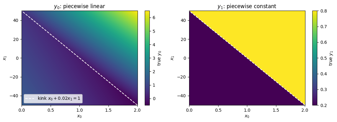
Output 0 is piecewise linear with a kink along an oblique line. Output 1 is an intensive property that is constant on each side of the kink, which is the case where we want constant leaves so that bilinear blending terms linearize exactly. Inputs live on very different scales, to show that the export undoes the internal standardization.

def truth(X):
    u = X[:, 0] + 0.02 * X[:, 1] - 1.0           # oblique kink
    y0 = np.where(u > 0, 3.0 * u, -1.0 * u) + 0.01 * X[:, 1]   # continuous across the kink
    y1 = np.where(u > 0, 0.8, 0.2)
    return np.stack([y0, y1], axis=1)

def truth_jac(X):
    u = X[:, 0] + 0.02 * X[:, 1] - 1.0
    J = np.zeros((X.shape[0], 2, 2))
    right = u > 0
    J[:, 0, 0] = np.where(right, 3.0, -1.0)
    J[:, 0, 1] = np.where(right, 3.0 * 0.02, -1.0 * 0.02) + 0.01
    return J  # output 1 is piecewise constant: zero Jacobian

rng = np.random.default_rng(0)
lo, hi = np.array([0.0, -50.0]), np.array([2.0, 50.0])
X_te = rng.uniform(lo, hi, (4000, 2))
Y_te = truth(X_te)

What the surrogate has to learn

The left panel is \(y_0\) over the design box: two planes meeting along the oblique kink (dashed). The right panel is \(y_1\), a step across the same line. A tree that puts one split on the dashed line can represent both outputs exactly with two affine leaves.

g0, g1 = np.meshgrid(np.linspace(lo[0], hi[0], 300), np.linspace(lo[1], hi[1], 300))
G = np.stack([g0.ravel(), g1.ravel()], axis=1)
TG = truth(G)
u0 = np.linspace(lo[1], hi[1], 2)

fig, axes = plt.subplots(1, 2, figsize=(11, 4))
for k, ax in enumerate(axes):
    im = ax.pcolormesh(g0, g1, TG[:, k].reshape(g0.shape), shading="auto", cmap="viridis")
    ax.plot(1.0 - 0.02 * u0, u0, "w--", lw=1.5, label="kink $x_0 + 0.02 x_1 = 1$")
    plt.colorbar(im, ax=ax, label=f"true $y_{k}$")
    ax.set(xlabel="$x_0$", ylabel="$x_1$", title=["$y_0$: piecewise linear", "$y_1$: piecewise constant"][k])
axes[0].legend(loc="lower left")
plt.tight_layout()
plt.show()

Affine vs constant leaves

60 training points. Everything below is hardened (hardening=True), so we compare the crisp models that would go into a MILP.

X = rng.uniform(lo, hi, (60, 2))
Y = truth(X) + 0.01 * rng.normal(size=(60, 2))
J = truth_jac(X)

common = dict(depth=2, n_epochs=300, batch_size=32, hardening=True, random_state=0)
models = {
    "constant": DifferentiableTreeRegressor(**common).fit(X, Y),
    "affine": DifferentiableTreeRegressor(leaf_type="affine", constant_outputs=[1], **common).fit(X, Y),
}
for name, mod in models.items():
    rmse = np.sqrt(np.mean((mod.predict(X_te, hard=True) - Y_te) ** 2, axis=0))
    print(f"{name:>9s}: hard RMSE y0={rmse[0]:.3f}  y1={rmse[1]:.3f}")

 constant: hard RMSE y0=0.762  y1=0.118
   affine: hard RMSE y0=0.023  y1=0.086

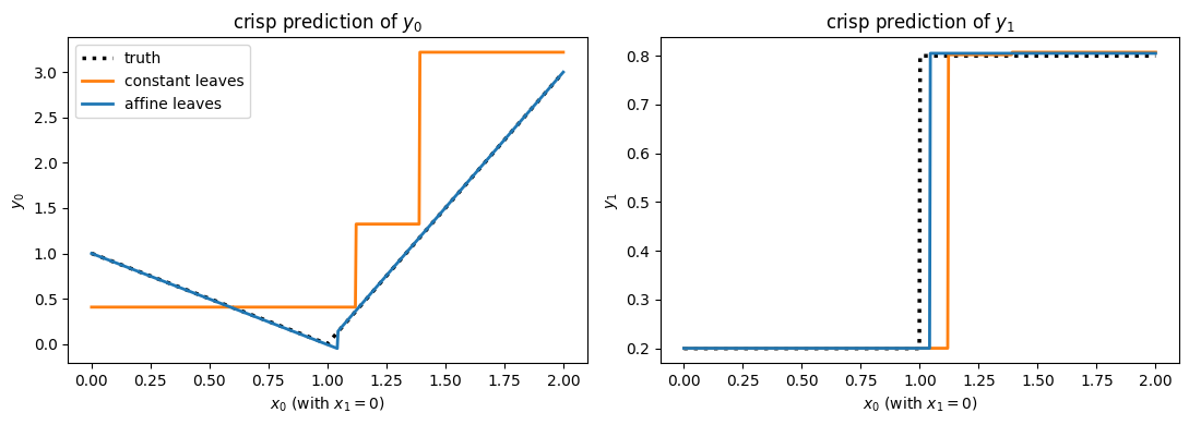
The printed RMSE hides how the two leaf types fail. Below, both models are evaluated along the line \(x_1 = 0\), which crosses the kink at \(x_0 = 1\). With a depth-2 tree there are only four leaves, so constant leaves approximate the two ramps of \(y_0\) with a coarse staircase. Affine leaves reproduce each ramp exactly and only need the split to sit on the kink. For \(y_1\) both leaf types are constant (we asked for constant_outputs=[1]), so they differ only in where the step lands.

xs = np.linspace(lo[0], hi[0], 600)
S0 = np.c_[xs, np.zeros_like(xs)]
fig, axes = plt.subplots(1, 2, figsize=(11, 4))
for k, ax in enumerate(axes):
    ax.plot(xs, truth(S0)[:, k], "k:", lw=2.5, label="truth")
    for name, c in (("constant", "C1"), ("affine", "C0")):
        ax.plot(xs, models[name].predict(S0, hard=True)[:, k], color=c, lw=2, label=f"{name} leaves")
    ax.set(xlabel="$x_0$ (with $x_1 = 0$)", ylabel=f"$y_{k}$", title=f"crisp prediction of $y_{k}$")
axes[0].legend()
plt.tight_layout()
plt.show()

Jacobian matching with very few samples

With 60 points the affine fit is already at the noise floor, so derivatives add little. They matter when samples are scarce. The cell below fits 5 random training sets each at \(n = 12\) and \(n = 24\), with and without dydx, and reports the median crisp RMSE on \(y_0\). Individual runs vary, which is why we take the median.

all_errs = {}
for n in (12, 24):
    errs = {"no dydx": [], "dydx": []}
    for seed in range(5):
        r = np.random.default_rng(100 + seed)
        Xn = r.uniform(lo, hi, (n, 2))
        Yn = truth(Xn) + 0.01 * r.normal(size=(n, 2))
        for name, dydx in (("no dydx", None), ("dydx", truth_jac(Xn))):
            mod = DifferentiableTreeRegressor(
                leaf_type="affine", constant_outputs=[1], validation_fraction=0.2, **common
            ).fit(Xn, Yn, dydx=dydx)
            errs[name].append(np.sqrt(np.mean((mod.predict(X_te, hard=True)[:, 0] - Y_te[:, 0]) ** 2)))
    all_errs[n] = errs
    print(f"n={n:2d}: median RMSE(y0) without dydx={np.median(errs['no dydx']):.3f}  "
          f"with dydx={np.median(errs['dydx']):.3f}")

n=12: median RMSE(y0) without dydx=0.106  with dydx=0.187

n=24: median RMSE(y0) without dydx=0.159  with dydx=0.156

fig, ax = plt.subplots(figsize=(6.5, 4))
for i, n in enumerate(all_errs):
    for j, (name, c) in enumerate((("no dydx", "C0"), ("dydx", "C3"))):
        xpos = i * 3 + j
        e = all_errs[n][name]
        ax.scatter(np.full(len(e), xpos) + np.linspace(-0.12, 0.12, len(e)), e, color=c, s=30,
                   label=name if i == 0 else None)
        ax.hlines(np.median(e), xpos - 0.3, xpos + 0.3, color=c, lw=2)
ax.set_xticks([0.5, 3.5], [f"n = {n}" for n in all_errs])
ax.set(ylabel="crisp RMSE of $y_0$ (test set)", title="Each dot is one training set; bars are medians")
ax.legend()
plt.tight_layout()
plt.show()

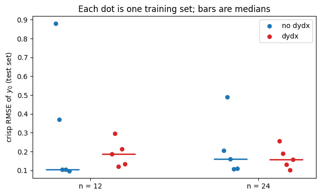
The medians hide the spread. Without dydx a few training sets give a badly placed kink and a large error (the outliers near 0.9 and 0.5); with dydx the worst case is much better even though the median is not. Derivatives make the fit more robust here rather than more accurate on average.

On this problem the derivatives do not help: at \(n = 12\) the median error is higher with dydx, and at \(n = 24\) it is about the same. The remaining error comes from where the tree places the kink, and the Jacobian term informs that only indirectly. It trains the leaf slopes, while the splits move only through the routing weights. In the test suite there is a case where dydx clearly helps (30 samples, kink along \(x_0 = 0\): crisp RMSE 0.41 → 0.17), so treat jacobian_weight as a hyperparameter and validate it on your data.

For the rest of the notebook we use the 60-point affine model, refit with the Jacobians.

m = DifferentiableTreeRegressor(leaf_type="affine", constant_outputs=[1], **common).fit(X, Y, dydx=J)

The hardening report

hardening_report_ compares soft and crisp predictions on the held-out validation slice, before and after hardening. A large rmse_gap (crisp minus soft) or a low mean_max_leaf_prob before hardening means the soft fit leans on blending leaves, which makes it a poor guide to the MILP model. soft_hard_gap(X, y) computes the same numbers on any data.

for stage in ("before", "after"):
    r = m.hardening_report_[stage]
    print(f"{stage:>6s}: rmse soft={np.round(r['rmse_soft'], 3)} hard={np.round(r['rmse_hard'], 3)} "
          f"gap={np.round(r['rmse_gap'], 3)}  max leaf prob={r['mean_max_leaf_prob']:.3f}")

gap = m.soft_hard_gap(X_te, Y_te)
print("test-set gap:", np.round(gap["rmse_gap"], 4), " routing agreement:", gap["routing_agreement"])

before: rmse soft=[0.009 0.009] hard=[0.009 0.009] gap=[-0. -0.]  max leaf prob=1.000
 after: rmse soft=[0.01  0.009] hard=[0.01  0.009] gap=[-0. -0.]  max leaf prob=1.000

test-set gap: [0.0021 0.0056]  routing agreement: 1.0

Soft vs hardened: what hardening changes

difftree trains a soft tree: every input reaches every leaf with some probability, and predict() blends the leaf models. A MILP can only use the crisp tree, predict(hard=True), which sends each input to one leaf by the sign of each split. Those two can be quite different models. The options are:

• hardening=False (the default): the soft tree is the fitted model. predict(hard=True) still works, but the leaves were never trained to be used on their own.

• hardening=True in the constructor, or model.harden(X, y) on an already fitted model: keep training while \(\gamma\) grows to gamma_hard (over n_hard_epochs), freeze the partition, refit each leaf by least squares on its own points (hard_ridge shrinks toward the soft values), and recalibrate the noise scale.

The two-output problem above is so easy that the soft tree is already almost crisp (max leaf probability 1.000 in the report), so the difference is invisible there. A smooth 1-D function shows it clearly. Below, the same depth-3 affine-leaf model is fitted to \(\sin 2x\) once without hardening, and then hardened.

import copy

r1 = np.random.default_rng(0)
x1 = r1.uniform(-2, 2, (300, 1))
y1 = np.sin(2 * x1[:, 0]) + 0.03 * r1.normal(size=300)
soft = DifferentiableTreeRegressor(depth=3, n_epochs=200, leaf_type="affine", gamma_max=2.0,
                                   random_state=0).fit(x1, y1)      # hardening=False
hard = copy.deepcopy(soft).harden(x1, y1)                          # same model, hardened

xg = np.linspace(-2, 2, 1500)[:, None]
fig, axes = plt.subplots(1, 3, figsize=(15, 4), gridspec_kw={"width_ratios": [1, 1, 0.8]})
for ax, mod, title in ((axes[0], soft, "hardening=False"), (axes[1], hard, "after harden()")):
    ax.scatter(x1[:, 0], y1, s=6, color="0.75")
    ax.plot(xg[:, 0], mod.predict(xg), color="C0", lw=3, alpha=0.6, label="soft: predict()")
    ax.plot(xg[:, 0], mod.predict(xg, hard=True), color="k", lw=1.3, label="crisp: predict(hard=True)")
    for c in np.sort(-mod.params_["b"] / mod.params_["W"][:, 0]) * mod.x_std_[0] + mod.x_mean_[0]:
        if -2 < c < 2:
            ax.axvline(c, color="C3", lw=0.6, alpha=0.5)
    g = mod.soft_hard_gap(x1, y1)
    ax.set(xlabel="x", ylabel="y", title=f"{title}\nRMSE soft {g['rmse_soft'][0]:.3f}, crisp {g['rmse_hard'][0]:.3f}")
axes[0].legend(loc="lower right", fontsize=9)
for mod, name, c in ((soft, "hardening=False", "C1"), (hard, "after harden()", "C2")):
    axes[2].plot(xg[:, 0], np.abs(mod.predict(xg) - mod.predict(xg, hard=True)), color=c, label=name)
axes[2].set(xlabel="x", ylabel="|soft - crisp|", title="Where the soft and crisp models differ")
axes[2].legend()
plt.tight_layout()
plt.show()

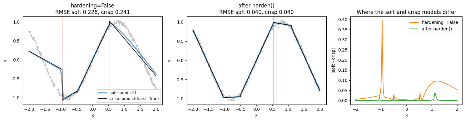
Red lines are the split locations. Without hardening, the soft model is smooth across each split because it blends neighbouring leaves, while the crisp model jumps there (largest differences in the right panel, right at the splits). Worse, neither fits well: the leaves were trained to be blended, so on its own each one is a poor local model. After harden() the splits are sharp, each leaf is refit on its own points, and soft and crisp agree almost everywhere. That crisp model is the one the MILP sees.

The hardening report quantifies the same thing on the validation slice. mean_max_leaf_prob near 1 means the soft tree is effectively crisp; rmse_gap is crisp minus soft error.

for name, mod in (("hardening=False", soft), ("after harden()", hard)):
    g = mod.soft_hard_gap(x1, y1)
    print(f"{name:>16s}: rmse soft={g['rmse_soft'][0]:.3f} crisp={g['rmse_hard'][0]:.3f} "
          f"gap={g['rmse_gap'][0]:+.3f}  max leaf prob={g['mean_max_leaf_prob']:.3f}  "
          f"routing agreement={g['routing_agreement']:.3f}")

 hardening=False: rmse soft=0.228 crisp=0.241 gap=+0.013  max leaf prob=0.829  routing agreement=0.997
  after harden(): rmse soft=0.040 crisp=0.040 gap=-0.001  max leaf prob=0.987  routing agreement=1.000

Leaf polytopes in original units

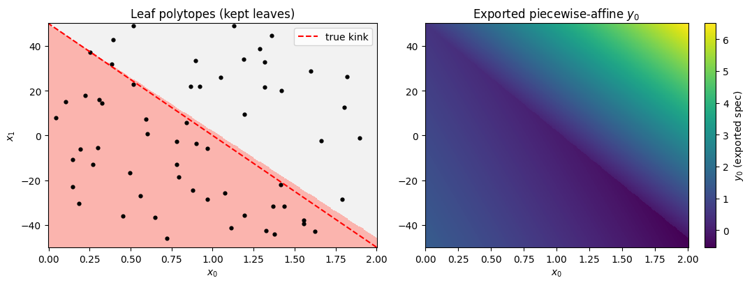
export.leaf_polytopes returns one region per leaf, intersected with an input box (by default the training-data box; here we pass the design box). One LP per leaf drops leaves with an empty interior. A depth-2 tree has 4 leaves, but the box often contains only some of them.

polys = export.leaf_polytopes(m, bounds=(lo, hi), X=X)
print(f"{len(polys)} non-empty leaves of {2 ** m.depth}")
for lp in polys:
    print(f"leaf {lp.leaf}: n_train={lp.n_samples}, path={lp.path}")
    print("   coef =", np.round(lp.coef, 4).tolist(), " intercept =", np.round(lp.intercept, 4).tolist())

2 non-empty leaves of 4
leaf 2: n_train=39, path=[(0, 'right'), (2, 'left')]
   coef = [[-1.0019, -0.01], [0.0, -0.0]]  intercept = [0.9971, 0.2004]
leaf 3: n_train=21, path=[(0, 'right'), (2, 'right')]
   coef = [[2.9988, 0.07], [0.0, 0.0]]  intercept = [-2.9958, 0.8051]

g0, g1 = np.meshgrid(np.linspace(lo[0], hi[0], 300), np.linspace(lo[1], hi[1], 300))
G = np.stack([g0.ravel(), g1.ravel()], axis=1)
region = np.full(G.shape[0], -1)
for k, lp in enumerate(polys):
    region[lp.contains(G)] = k

fig, axes = plt.subplots(1, 2, figsize=(11, 4.2))
axes[0].pcolormesh(g0, g1, region.reshape(g0.shape), cmap="Pastel1", shading="auto")
axes[0].scatter(X[:, 0], X[:, 1], s=12, c="k")
u0 = np.linspace(lo[1], hi[1], 2)
axes[0].plot(1.0 - 0.02 * u0, u0, "r--", label="true kink")
axes[0].set(xlabel="$x_0$", ylabel="$x_1$", title="Leaf polytopes (kept leaves)")
axes[0].legend(loc="upper right")

pred = export.predict_spec(export.to_spec(m, bounds=(lo, hi)), G)[:, 0]
im = axes[1].pcolormesh(g0, g1, pred.reshape(g0.shape), shading="auto")
plt.colorbar(im, ax=axes[1], label="$y_0$ (exported spec)")
axes[1].set(xlabel="$x_0$", title="Exported piecewise-affine $y_0$")
plt.tight_layout()
plt.show()

jax-ldt JSON spec

export.to_json writes the solver-neutral v1 spec of jax-ldt. Each oblique split is a lifted column of transform_matrix ([I | a_1 ... a_k]), so jax_ldt.export.from_json and its discopt adapter (embed_in_discopt_model) can consume the model directly. export.predict_spec evaluates a spec in NumPy and reproduces predict(hard=True) to round-off inside the box.

s = export.to_json(m, bounds=(lo, hi))
spec = json.loads(s)
print("kind:", spec["kind"], "| nodes:", spec["tree"]["node_count"],
      "| lifted features:", spec["n_features_transformed"])
X_box = rng.uniform(lo, hi, (2000, 2))
err = np.abs(export.predict_spec(spec, X_box) - m.predict(X_box, hard=True)).max()
print(f"max |spec - predict(hard=True)| = {err:.2e}")

kind: hyperplane_tree | nodes: 3 | lifted features: 3
max |spec - predict(hard=True)| = 1.78e-15

With jax-ldt (and discopt) installed, the same string embeds in a MILP:

import jax; jax.config.update("jax_enable_x64", True)
import discopt
from jax_ldt import from_json
from jax_ldt.export import embed_in_discopt_model

tree = from_json(s)
mdl = discopt.Model("surrogate")
x = mdl.continuous("x", shape=(2,), lb=lo, ub=hi)
y = embed_in_discopt_model(tree, mdl, x)
mdl.minimize(y[0])
result = mdl.solve()

The MILP treats leaf polytopes as closed sets, so an optimum can sit on a split boundary and use either neighbouring leaf’s model there. See jax-ldt’s boundary_eps option if that matters.

Split boundaries: jumps and repairing a MILP solution

A crisp piecewise-affine tree can jump across a split. The MILP treats leaf polytopes as closed, so its optimum can land on a boundary and use either neighbouring leaf’s model, while predict(hard=True) sends boundary points left. export.boundary_jumps measures how large the jumps are on every shared facet in the box.

for j in export.boundary_jumps(m, bounds=(lo, hi)):
    print(f"node {j['node']}: leaves {j['left']}|{j['right']}  max jump per output = {np.round(j['max_jump'], 3)}")

node 2: leaves 2|3  max jump per output = [0.348 0.605]

Suppose a MILP returns a point on this boundary where the jump is largest. At a boundary point the solver can report either neighbouring leaf, and its objective uses that leaf’s model (in practice, read the chosen leaf from the binaries with export.leaf_from_binaries(spec, z)). Below we take the leaf that predict(hard=True) does not use at that exact point, which is the case that causes trouble. export.repair_solution moves the point \(\delta\) (standardized units) into the chosen leaf, after which crisp prediction and the MILP agree.

j = export.boundary_jumps(m, bounds=(lo, hi))[0]
x_boundary = j["worst_point"][0]   # where output 0 jumps the most
polys = {lp.leaf: lp for lp in export.leaf_polytopes(m, bounds=(lo, hi))}
vals = {leaf: polys[leaf].predict(x_boundary[None])[0, 0] for leaf in (j["left"], j["right"])}
routed = m.apply(x_boundary[None])[0]
chosen = j["right"] if routed == j["left"] else j["left"]   # the solver's choice
x_fixed = export.repair_solution(m, x_boundary, chosen, bounds=(lo, hi))
print(f"MILP objective (leaf {chosen})       : {vals[chosen]:.4f}")
print(f"predict(hard=True) at boundary  : {m.predict(x_boundary[None], hard=True)[0, 0]:.4f}  (leaf {m.apply(x_boundary[None])[0]})")
print(f"predict(hard=True) after repair : {m.predict(x_fixed[None], hard=True)[0, 0]:.4f}  (leaf {m.apply(x_fixed[None])[0]})")
print(f"moved by {np.max(np.abs((x_fixed - x_boundary) / m.x_std_)):.1e} (standardized units)")

MILP objective (leaf 3)       : -0.2008
predict(hard=True) at boundary  : -0.5486  (leaf 2)
predict(hard=True) after repair : -0.2008  (leaf 3)
moved by 2.2e-06 (standardized units)

The picture: a slice through x_boundary across the split. The dotted lines extend each leaf’s affine model past the boundary. The MILP’s objective uses the chosen leaf’s line (orange dot), while predict(hard=True) at the exact boundary point uses the other one (blue square). repair_solution nudges the point a distance \(\delta\) to the chosen side (shown exaggerated here; the real move is about \(10^{-6}\)).

node_w = m.params_["W"][j["node"]]
step = (node_w / np.linalg.norm(node_w)) * m.x_std_        # unit step in standardized units
t = np.linspace(-0.3, 0.3, 1200)
S = x_boundary[None, :] + t[:, None] * step[None, :]

fig, ax = plt.subplots(figsize=(8, 4.5))
for leaf in (j["left"], j["right"]):
    ax.plot(t, polys[leaf].predict(S)[:, 0], ":", color="0.6", lw=1.2)
ax.plot(t, truth(S)[:, 0], color="C1", lw=1, alpha=0.6, label="truth")
ax.plot(t, m.predict(S, hard=True)[:, 0], color="k", lw=2.5, label="crisp model")
ax.plot(0, vals[chosen], "o", ms=11, color="C1", mec="k", label=f"MILP objective (leaf {chosen})")
ax.plot(0, m.predict(x_boundary[None], hard=True)[0, 0], "s", ms=10, color="C0", mec="k",
        label="predict(hard=True) at x_boundary")
ax.annotate("", xy=(0.03, vals[chosen]), xytext=(0, vals[chosen]),
            arrowprops=dict(arrowstyle="->", color="C2", lw=2))
ax.text(0.035, vals[chosen] - 0.03, "repair_solution (δ exaggerated)", color="C2", va="top")
ax.axvline(0, color="0.8", lw=0.8)
ax.set(xlabel="distance across the split (standardized x)", ylabel="$y_0$")
ax.legend(loc="upper left", fontsize=9)
plt.tight_layout()
plt.show()

Jumps vs continuity

There are three ways to harden the same data:

• discontinuous (default): every leaf is fitted on its own, so neighbouring leaves can disagree at a split.

• continuous, untied (continuous=True): neighbouring leaves must agree on each shared facet. On an oblique tree this is expensive. Wherever a deeper split meets a parent boundary (a T-junction), both leaves of that split must match the same neighbour, which forces them to merge unless the two hyperplanes coincide. Each kink is also pinned to wherever the learned split happens to sit.

• continuous, tied (tied_splits=True, continuous=True): all nodes at a depth share one hyperplane, so every junction is a crossing. A continuous function on that partition is exactly a hinging-hyperplanes model, \(\theta_0 \cdot [1, x] + \sum_d c_d \max(0, w_d \cdot x + b_d)\), which hardening fits directly while moving the hyperplanes to reduce the error (refine_splits). It is continuous everywhere, not only inside the box.

The first panel takes a slice through the oblique kink of this notebook’s function. The second uses a 3-input function with two kinks, \(|x_0| + x_1 + \max(x_2, 0)\), sliced along \(x_0\).

variants = {
    "discontinuous": dict(),
    "continuous, untied": dict(continuous=True),
    "continuous, tied": dict(continuous=True, tied_splits=True),
}
aff = dict(leaf_type="affine", constant_outputs=[1], **common)
fits2d = {name: DifferentiableTreeRegressor(**aff, **kw).fit(X, Y) for name, kw in variants.items()}

f3 = lambda Z: np.abs(Z[:, 0]) + Z[:, 1] + np.maximum(Z[:, 2], 0)
r3 = np.random.default_rng(1)
X3 = r3.uniform(-2, 2, (600, 3))
y3 = f3(X3) + 0.02 * r3.normal(size=600)
X3_te = r3.uniform(-2, 2, (5000, 3))
kw3 = dict(depth=3, n_epochs=80, leaf_type="affine", hardening=True, n_hard_epochs=20, random_state=0)
fits3d = {name: DifferentiableTreeRegressor(**kw3, **kw).fit(X3, y3) for name, kw in variants.items()}

print(f"{'':>20s} {'2-D kink (y0)':>24s}   {'3-D two kinks':>24s}")
print(f"{'':>20s} {'RMSE':>10s} {'max jump':>12s}   {'RMSE':>10s} {'max jump':>12s}")
for name in variants:
    a, b = fits2d[name], fits3d[name]
    ra = np.sqrt(np.mean((a.predict(X_te, hard=True)[:, 0] - Y_te[:, 0]) ** 2))
    rb = np.sqrt(np.mean((b.predict(X3_te, hard=True) - f3(X3_te)) ** 2))
    print(f"{name:>20s} {ra:10.3f} {a.hardening_report_['max_boundary_jump'][0]:12.2e}   "
          f"{rb:10.3f} {b.hardening_report_['max_boundary_jump'][0]:12.2e}")

                                2-D kink (y0)              3-D two kinks
                           RMSE     max jump         RMSE     max jump
       discontinuous      0.023     3.58e-01        0.049     3.60e-01
  continuous, untied      0.073     5.38e-16        0.583     1.11e-15
    continuous, tied      0.007     3.50e-15        0.004     3.22e-16

styles = {"discontinuous": ("C0", "-"), "continuous, untied": ("C1", "--"), "continuous, tied": ("C2", "-")}

def worst_slice(model, half_width=1.0, n=2000):
    """Line through the discontinuous model's worst jump, across that split.
    Returns (t, points): t is the signed distance in standardized x units."""
    j = export.boundary_jumps(model)[0]
    x_w = j["worst_point"][0]
    w = model.params_["W"][j["node"]]
    step = (w / np.linalg.norm(w)) * model.x_std_   # unit step in standardized units
    t = np.linspace(-half_width, half_width, n)
    return t, x_w[None, :] + t[:, None] * step[None, :]

fig, axes = plt.subplots(1, 2, figsize=(12, 4.2))
for ax, fits, f_true, title in (
    (axes[0], fits2d, lambda Z: truth(Z)[:, 0], "2-D oblique kink ($y_0$), depth 2"),
    (axes[1], fits3d, f3, "$|x_0| + x_1 + \\max(x_2, 0)$, depth 3"),
):
    t, S = worst_slice(fits["discontinuous"])
    ax.plot(t, f_true(S), "k:", lw=2, label="truth")
    for name, mod in fits.items():
        c, ls = styles[name]
        pred = mod.predict(S, hard=True)
        ax.plot(t, pred[:, 0] if pred.ndim == 2 else pred, color=c, ls=ls, label=name)
    ax.axvline(0, color="0.7", lw=0.8)
    ax.set(xlabel="distance across the worst split (standardized x)", ylabel="prediction", title=title)
    ax.legend()
plt.tight_layout()
plt.show()

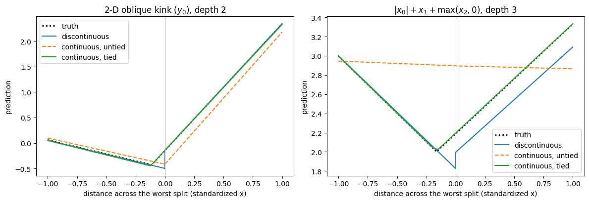
Each slice crosses the split where the discontinuous tree’s jump is largest (the grey line). There the blue curve steps, which is the jump a MILP can exploit. The green curve crosses smoothly and follows the truth. The orange curve is continuous but has lost most of the shape.

On these problems the tied continuous model has no jumps and is at least as accurate as the discontinuous tree. The untied continuous model is jump-free but much less accurate, for the reasons above. Tied splits do restrict the partition (one hyperplane per depth). On smooth functions with no kink structure (e.g. \(\sin 2x\) or a Gaussian bump) the README’s comparison shows the tied continuous model roughly matching the discontinuous tree, sometimes slightly worse, so check soft_hard_gap and boundary_jumps on your own data.