Failure modes: seeds, local inverse design, missing epistemic uncertainty, readability

The deck lists four limitations that are about behaviour rather than cost (the cost ones are in scaling.ipynb):

1. Non-convex training. The result depends on the random seed.

2. Local inverse design. \(\log p(y^* \mid x)\) is multimodal, and gradient ascent finds the mode nearest its start.

3. Single tree, aleatoric-heavy uncertainty. The predictive spread comes from leaf noise and routing ambiguity, with no uncertainty about the parameters themselves, so it does not grow away from the data.

4. Less interpretable. Oblique, soft splits are weighted sums of several inputs.

Each section below measures one of them and suggests a mitigation.

from pathlib import Path

import matplotlib.pyplot as plt
import numpy as np
from sklearn.datasets import make_friedman1
from sklearn.tree import DecisionTreeRegressor

from difftree import DifferentiableTreeRegressor

FIG = Path("../presentation/figures")
summary = {}          # numbers reused in the summary figure

1. Seed sensitivity

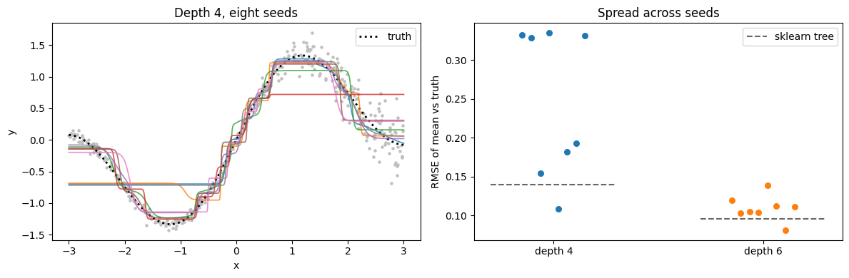
The 1-D problem from the deck: \(f(x) = \sin 1.5x + 0.3x\) with noise that grows for \(x > 0\), 400 training points. We fit the same configuration with 8 seeds at depths 4 and 6 and measure the RMSE of the predictive mean against the true \(f\). The validation NLL that difftree reports after fitting is available without the truth, so we also check whether choosing the seed with the best validation score picks a good model.

rng = np.random.default_rng(0)
x1 = np.sort(rng.uniform(-3, 3, 400))[:, None]
f1 = lambda x: np.sin(1.5 * x) + 0.3 * x
y1 = f1(x1[:, 0]) + rng.normal(0, 0.05 + 0.25 * (x1[:, 0] > 0) * np.abs(x1[:, 0]) / 3)
xg = np.linspace(-3, 3, 600)[:, None]
xv = rng.uniform(-3, 3, (400, 1))
yv = f1(xv[:, 0]) + rng.normal(0, 0.05 + 0.25 * (xv[:, 0] > 0) * np.abs(xv[:, 0]) / 3)

seeds = range(8)
seed_fits = {}
for D in (4, 6):
    for s in seeds:
        m = DifferentiableTreeRegressor(depth=D, n_epochs=150, random_state=s).fit(x1, y1)
        rmse = np.sqrt(np.mean((m.predict(xg) - f1(xg[:, 0])) ** 2))
        val_score = m.score(xv, yv)          # R^2 on fresh data, no truth needed
        seed_fits[D, s] = (m, rmse, val_score)
    r = [seed_fits[D, s][1] for s in seeds]
    best = max(seeds, key=lambda s: seed_fits[D, s][2])
    print(f"depth {D}: RMSE vs truth min {min(r):.3f}  median {np.median(r):.3f}  max {max(r):.3f}  "
          f"| seed picked by held-out R^2: {best} (RMSE {seed_fits[D, best][1]:.3f})")
sk_rmse = {D: np.sqrt(np.mean((DecisionTreeRegressor(max_depth=D, random_state=0).fit(x1, y1).predict(xg)
                               - f1(xg[:, 0])) ** 2)) for D in (4, 6)}
print("sklearn tree RMSE vs truth:", {D: round(v, 3) for D, v in sk_rmse.items()})

depth 4: RMSE vs truth min 0.108  median 0.261  max 0.335  | seed picked by held-out R^2: 4 (RMSE 0.108)

depth 6: RMSE vs truth min 0.081  median 0.108  max 0.138  | seed picked by held-out R^2: 6 (RMSE 0.081)
sklearn tree RMSE vs truth: {4: np.float64(0.14), 6: np.float64(0.095)}

fig, axes = plt.subplots(1, 2, figsize=(12, 4))
ax = axes[0]
ax.scatter(x1[:, 0], y1, s=5, color="0.75")
ax.plot(xg[:, 0], f1(xg[:, 0]), "k:", lw=2, label="truth")
for s in seeds:
    ax.plot(xg[:, 0], seed_fits[4, s][0].predict(xg), lw=1.2, alpha=0.8)
ax.set(xlabel="x", ylabel="y", title="Depth 4, eight seeds")
ax.legend()
ax = axes[1]
for i, D in enumerate((4, 6)):
    r = [seed_fits[D, s][1] for s in seeds]
    ax.scatter(np.full(len(r), i) + np.linspace(-0.15, 0.15, len(r)), r, s=30, color=f"C{i}")
    ax.hlines(sk_rmse[D], i - 0.3, i + 0.3, color="0.4", ls="--", label="sklearn tree" if i == 0 else None)
ax.set_xticks([0, 1], ["depth 4", "depth 6"])
ax.set(ylabel="RMSE of mean vs truth", title="Spread across seeds")
ax.legend()
plt.tight_layout()
plt.show()
summary["seeds"] = {D: [seed_fits[D, s][1] for s in seeds] for D in (4, 6)}

2. Inverse design is local

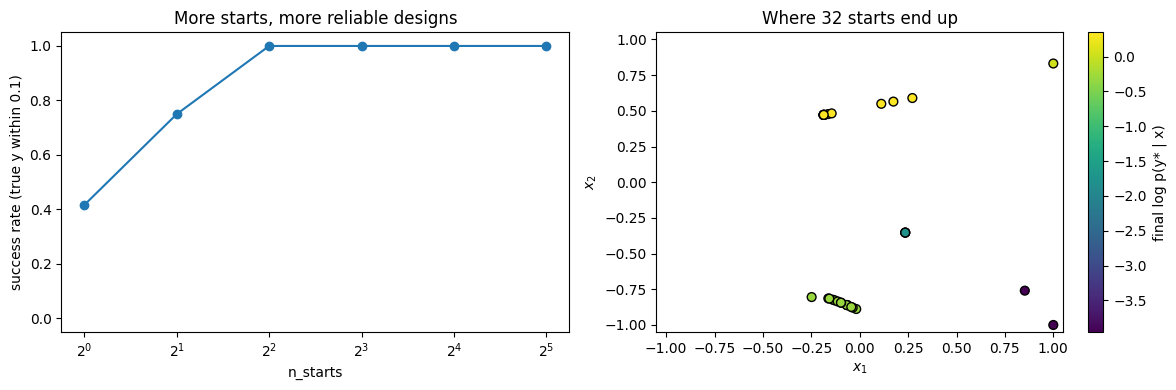
The two-output problem from the deck: three inputs in \([-1, 1]^3\), target \(y^* = (1.8, 1.0)\). We run inverse_design with 1 to 32 starts, repeated with 12 random states each, and score each answer against the true function (not the surrogate): success means both true outputs are within 0.1 of the target. We also count how many distinct optima the 32-start run finds (final points more than 0.2 apart with log-likelihood within 2 of the best).

def true_means(X):
    a, b_, c_ = X[:, 0], X[:, 1], X[:, 2]
    y_1 = 1.5 + 0.8 * np.tanh(2.0 * a - c_) - 0.5 * b_
    y_2 = 0.4 * y_1 + 0.6 * np.cos(1.5 * b_) + 0.2 * c_
    return np.stack([y_1, y_2], axis=1)

r2 = np.random.default_rng(0)
X2 = r2.uniform(-1, 1, (1500, 3)); Y2t = true_means(X2)
Y2 = Y2t + r2.normal(0, np.stack([0.05 + 0.10 * np.abs(Y2t[:, 0]), 0.05 + 0.08 * np.abs(Y2t[:, 1])], 1))
mm = DifferentiableTreeRegressor(depth=5, n_epochs=150, gamma_max=5.0, delta_gamma=0.05,
                                 sigma_init=0.5, random_state=0).fit(X2, Y2)

target = np.array([1.8, 1.0])
box = (np.full(3, -1.0), np.full(3, 1.0))
starts = [1, 2, 4, 8, 16, 32]
success, true_err = [], []
for k in starts:
    ok, errs = [], []
    for rs in range(12):
        xb, _, _, _ = mm.inverse_design({0: 1.8, 1: 1.0}, n_starts=k, n_steps=400, bounds=box, random_state=rs)
        e = np.max(np.abs(true_means(xb[None])[0] - target))
        ok.append(e < 0.1); errs.append(e)
    success.append(np.mean(ok)); true_err.append(np.median(errs))
    print(f"n_starts {k:2d}: success {success[-1]:.2f}  median max|y_true - y*| {true_err[-1]:.3f}")

xb, llb, x_all, lls = mm.inverse_design({0: 1.8, 1: 1.0}, n_starts=32, n_steps=400, bounds=box, random_state=0)
good = np.where(lls > llb - 2)[0]
reps = []
for i in good[np.argsort(-lls[good])]:
    if all(np.max(np.abs(x_all[i] - x_all[j])) > 0.2 for j in reps):
        reps.append(i)
print(f"32 starts: {len(good)} end within 2 log-units of the best, forming {len(reps)} distinct optima:")
for i in reps:
    print(f"   x = {np.round(x_all[i], 2)}  log p = {lls[i]:.2f}  true y = {np.round(true_means(x_all[i][None])[0], 3)}")

n_starts  1: success 0.42  median max|y_true - y*| 0.124

n_starts  2: success 0.75  median max|y_true - y*| 0.090

n_starts  4: success 1.00  median max|y_true - y*| 0.090

n_starts  8: success 1.00  median max|y_true - y*| 0.090

n_starts 16: success 1.00  median max|y_true - y*| 0.090

n_starts 32: success 1.00  median max|y_true - y*| 0.090

32 starts: 27 end within 2 log-units of the best, forming 6 distinct optima:
   x = [-0.19  0.47 -1.  ]  log p = 0.35  true y = [1.709 0.94 ]
   x = [ 0.11  0.55 -1.  ]  log p = 0.33  true y = [1.898 0.967]
   x = [ 1.    0.83 -0.28]  log p = 0.03  true y = [1.867 0.882]
   x = [-0.13 -0.83 -0.35]  log p = -0.31  true y = [1.988 0.919]
   x = [-0.04 -0.88 -0.14]  log p = -0.31  true y = [1.991 0.919]
   x = [-0.25 -0.8  -0.64]  log p = -0.32  true y = [2.013 0.892]

fig, axes = plt.subplots(1, 2, figsize=(12, 4))
ax = axes[0]
ax.semilogx(starts, success, "o-", base=2)
ax.set(xlabel="n_starts", ylabel="success rate (true y within 0.1)", ylim=(-0.05, 1.05),
       title="More starts, more reliable designs")
ax = axes[1]
sc = ax.scatter(x_all[:, 0], x_all[:, 1], c=lls, cmap="viridis", s=40, edgecolor="k")
plt.colorbar(sc, ax=ax, label="final log p(y* | x)")
ax.set(xlabel="$x_1$", ylabel="$x_2$", xlim=(-1.05, 1.05), ylim=(-1.05, 1.05),
       title="Where 32 starts end up")
plt.tight_layout()
plt.show()
summary["inverse"] = (starts, success, x_all, lls)

3. No epistemic uncertainty away from the data

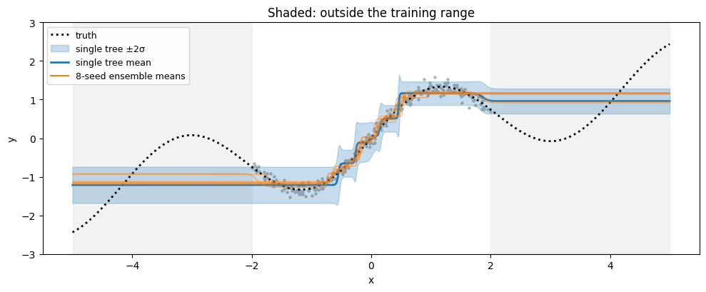
Train on \(x \in [-2, 2]\) only and predict on \([-5, 5]\). A model with parameter uncertainty (a GP, a Bayesian model, or an ensemble) would widen its intervals outside the training range. A single difftree cannot: outside the data every input routes to an edge leaf, which predicts that leaf’s mean and noise. We compare the single model’s \(\pm 2\sigma\) band with the spread of the means of 8 trees trained from different seeds, a cheap ensemble.

r3 = np.random.default_rng(3)
xt = r3.uniform(-2, 2, (300, 1))
f3 = lambda x: np.sin(1.5 * x) + 0.3 * x
yt = f3(xt[:, 0]) + 0.1 * r3.normal(size=300)
xe = np.linspace(-5, 5, 800)[:, None]

ens = [DifferentiableTreeRegressor(depth=4, n_epochs=150, random_state=s).fit(xt, yt) for s in range(8)]
mean0, std0 = ens[0].predict(xe, return_std=True)
means = np.stack([e.predict(xe) for e in ens])
inside = np.abs(xe[:, 0]) <= 2
err = np.abs(mean0 - f3(xe[:, 0]))
print(f"single model: mean sigma inside {std0[inside].mean():.3f}, outside {std0[~inside].mean():.3f}")
print(f"              mean |error| inside {err[inside].mean():.3f}, outside {err[~inside].mean():.3f}")
print(f"ensemble:     std of means inside {means.std(0)[inside].mean():.3f}, outside {means.std(0)[~inside].mean():.3f}")
cover = np.mean(np.abs(mean0 - f3(xe[:, 0]))[~inside] <= 2 * std0[~inside])
print(f"fraction of the true curve inside the single model's 2-sigma band, outside the data: {cover:.2f}")

single model: mean sigma inside 0.202, outside 0.198
              mean |error| inside 0.123, outside 0.792
ensemble:     std of means inside 0.060, outside 0.108
fraction of the true curve inside the single model's 2-sigma band, outside the data: 0.17

fig, ax = plt.subplots(figsize=(10, 4.2))
ax.axvspan(-5, -2, color="0.95"); ax.axvspan(2, 5, color="0.95")
ax.scatter(xt[:, 0], yt, s=5, color="0.7")
ax.plot(xe[:, 0], f3(xe[:, 0]), "k:", lw=2, label="truth")
ax.fill_between(xe[:, 0], mean0 - 2 * std0, mean0 + 2 * std0, color="C0", alpha=0.25, label="single tree ±2σ")
ax.plot(xe[:, 0], mean0, color="C0", lw=2, label="single tree mean")
for mu in means[1:]:
    ax.plot(xe[:, 0], mu, color="C1", lw=0.8, alpha=0.6)
ax.plot([], [], color="C1", label="8-seed ensemble means")
ax.set(xlabel="x", ylabel="y", ylim=(-3, 3), title="Shaded: outside the training range")
ax.legend(loc="upper left", fontsize=9)
plt.tight_layout()
plt.show()
summary["extrap"] = (xt, yt, xe, f3, mean0, std0, means)

4. Oblique splits mix several inputs

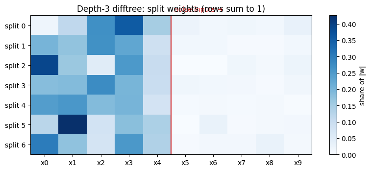
Friedman #1 with 10 inputs, of which only \(x_0 \dots x_4\) matter. Below are the absolute split weights \(|w_i|\) of a depth-3 difftree (7 splits, standardized inputs), each row normalised to sum to one, next to the one input each scikit-learn split uses. A classic split reads as “\(x_3 < 0.42\)”; an oblique split is a weighted sum of inputs. The effective number of inputs per split is \(1 / \sum_j \tilde w_j^2\) for the normalised weights \(\tilde w\): 1 for an axis-aligned split, 10 for equal weights on all ten.

Xf, yf = make_friedman1(n_samples=3000, n_features=10, noise=0.5, random_state=0)
mf = DifferentiableTreeRegressor(depth=3, n_epochs=150, random_state=0).fit(Xf, yf)
Wabs = np.abs(mf.params_["W"])                         # standardized inputs: comparable scales
Wn = Wabs / Wabs.sum(1, keepdims=True)
eff = 1.0 / (Wn ** 2).sum(1)                           # effective number of inputs per split
sk3 = DecisionTreeRegressor(max_depth=3, random_state=0).fit(Xf, yf)
print("effective inputs per difftree split:", np.round(eff, 1))
print("share of |w| on the 5 noise inputs:  ", np.round(Wn[:, 5:].sum(1), 2))
print("sklearn split features:", [int(f) for f in sk3.tree_.feature if f >= 0])

effective inputs per difftree split: [4.3 5.  3.9 5.1 4.8 3.9 4.8]
share of |w| on the 5 noise inputs:   [0.1  0.04 0.05 0.06 0.03 0.05 0.06]
sklearn split features: [3, 1, 4, 0, 0, 4, 1]

fig, ax = plt.subplots(figsize=(8, 3.6))
im = ax.imshow(Wn, cmap="Blues", aspect="auto", vmin=0)
plt.colorbar(im, ax=ax, label="share of |w|")
ax.set_xticks(range(10), [f"x{j}" for j in range(10)])
ax.set_yticks(range(Wn.shape[0]), [f"split {i}" for i in range(Wn.shape[0])])
ax.axvline(4.5, color="C3", lw=1.5)
ax.text(4.6, -0.7, "noise inputs →", color="C3", fontsize=10)
ax.set_title("Depth-3 difftree: split weights (rows sum to 1)")
plt.tight_layout()
plt.show()
summary["weights"] = Wn

Summary figure for the deck

fig, axes = plt.subplots(1, 4, figsize=(19, 4.2))
ax = axes[0]
for i, D in enumerate((4, 6)):
    r = summary["seeds"][D]
    ax.scatter(np.full(len(r), i) + np.linspace(-0.15, 0.15, len(r)), r, s=30, color=f"C{i}")
    ax.hlines(sk_rmse[D], i - 0.3, i + 0.3, color="0.4", ls="--", label="sklearn tree" if i == 0 else None)
ax.set_xticks([0, 1], ["depth 4", "depth 6"]); ax.set_xlim(-0.6, 1.6)
ax.legend(fontsize=9)
ax.set(ylabel="RMSE vs truth", title="Seed sensitivity (8 seeds)")

ax = axes[1]
st, succ, xa, ll = summary["inverse"]
ax.semilogx(st, succ, "o-", base=2)
ax.set(xlabel="n_starts", ylabel="success rate", ylim=(-0.05, 1.05), title="Inverse design needs multi-start")

ax = axes[2]
xt_, yt_, xe_, f_, m0, s0, ms = summary["extrap"]
ax.axvspan(-5, -2, color="0.93"); ax.axvspan(2, 5, color="0.93")
ax.plot(xe_[:, 0], f_(xe_[:, 0]), "k:", lw=2, label="truth")
ax.fill_between(xe_[:, 0], m0 - 2 * s0, m0 + 2 * s0, color="C0", alpha=0.25, label="±2σ")
ax.plot(xe_[:, 0], m0, color="C0", lw=2, label="mean")
ax.set(xlabel="x", ylim=(-3, 3), title="σ does not grow off the data")
ax.legend(fontsize=9, loc="upper left")

ax = axes[3]
im = ax.imshow(summary["weights"], cmap="Blues", aspect="auto", vmin=0)
ax.set_xticks(range(10), [f"x{j}" for j in range(10)], fontsize=8)
ax.axvline(4.5, color="C3", lw=1.5)
ax.set(ylabel="split", title="Each split mixes 4 to 5 inputs")
plt.tight_layout()
fig.savefig(FIG / "failure_modes.png", dpi=150)
plt.show()

What this shows

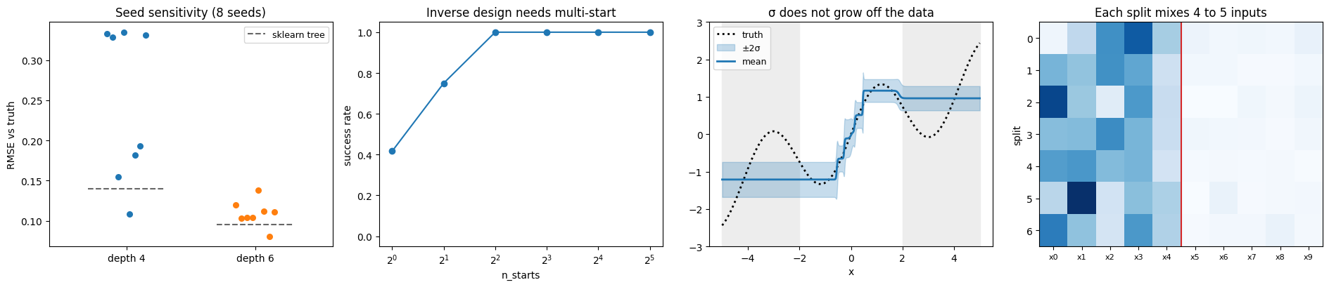
Seeds. At depth 4 the eight seeds give RMSE from 0.11 to 0.34 against the truth, a factor of three, and half of them are worse than a greedy scikit-learn tree of the same depth (0.14). The bad seeds park leaves on flat plateaus and miss whole sections of the curve. Depth 6 is far more stable (0.08 to 0.14) because spare leaves make up for badly placed splits. Choosing the seed by \(R^2\) on held-out data picked the best seed at both depths, so the practical fix is cheap: fit several seeds and keep the best on validation data.

Inverse design. One start succeeds only 42% of the time; four or more starts succeeded in all 12 repeats here. The 32-start run ends in six distinct optima spread over the box, with nearly equal likelihood, so the problem is genuinely multimodal and a single gradient ascent finds whichever basin it starts in. The remaining error of about 0.09 is the surrogate’s own error, not the optimizer’s. Use n_starts of 16 or more and look at x_all, which often holds useful alternative designs.

Extrapolation. The single tree’s \(\sigma\) is the same inside and outside the training range (about 0.20), while its error grows from 0.12 to 0.79. Outside the data the \(2\sigma\) band covers only 17% of the true curve. The 8-seed ensemble’s spread does grow outside (0.06 to 0.11), but far less than the error. Neither is a substitute for keeping queries inside the data, so check that inputs are in the training box before trusting an interval.

Readability. Each split mixes about 4 to 5 inputs, compared with exactly one for the scikit-learn tree. Training does learn to ignore the five noise inputs (3 to 10% of the weight), so the weights are informative, but a split is a hyperplane rather than a threshold. Shallow trees, or reading off the dominant weights of each split, are the practical compromise.