Multivariate UQ + cross-conditioning + inverse design
We fit a single DifferentiableTreeRegressor to a synthetic 2-output materials dataset,
then exercise three capabilities that fall out of the multivariate Gaussian-mixture
structure:
Joint marginal prediction \(p(\mathbf{y} \mid \mathbf{x})\) with full covariance.
Cross-conditioning: \(p(y_2 \mid \mathbf{x}, y_1)\) in closed form via Schur complements.
Inverse design: gradient-ascent over \(\mathbf{x}\) to maximize \(\log p(\mathbf{y}_{\text{target}} \mid \mathbf{x})\).
Synthetic problem
Two correlated material properties depending on three composition variables. The problem is set up so that \(y_1\) and \(y_2\) are non-trivially related through the inputs (not via an additive correlation in the noise), exactly the regime where conditioning should tighten uncertainty about \(y_2\) once \(y_1\) is observed.
import numpy as np
import matplotlib.pyplot as plt
from sklearn.model_selection import train_test_split

from difftree import DifferentiableTreeRegressor

rng = np.random.default_rng(0)
def true_means(X):
    x1, x2, x3 = X[:, 0], X[:, 1], X[:, 2]
    y1 = 1.5 + 0.8 * np.tanh(2.0 * x1 - x3) - 0.5 * x2
    y2 = 0.4 * y1 + 0.6 * np.cos(1.5 * x2) + 0.2 * x3
    return np.stack([y1, y2], axis=1)


def true_noise(Y_true):
    s1 = 0.05 + 0.10 * np.abs(Y_true[:, 0])
    s2 = 0.05 + 0.08 * np.abs(Y_true[:, 1])
    return np.stack([s1, s2], axis=1)


n = 1500
X = rng.uniform(-1.0, 1.0, (n, 3))
Y_true = true_means(X)
S_true = true_noise(Y_true)
Y = Y_true + rng.normal(0, S_true)

X_tr, X_te, Y_tr, Y_te = train_test_split(X, Y, test_size=300, random_state=0)
Yt_te = true_means(X_te)
St_te = true_noise(Yt_te)

print(f'train: {X_tr.shape[0]}, test: {X_te.shape[0]}')
print(f'y1 range: [{Y[:, 0].min():.2f}, {Y[:, 0].max():.2f}]')
print(f'y2 range: [{Y[:, 1].min():.2f}, {Y[:, 1].max():.2f}]')
print(f'corr(y1, y2): {np.corrcoef(Y_true[:, 0], Y_true[:, 1])[0, 1]:.3f}')
train: 1200, test: 300
y1 range: [0.15, 3.19]
y2 range: [0.04, 1.87]
corr(y1, y2): 0.747
Fit
model = DifferentiableTreeRegressor(
    depth=5, n_epochs=150, batch_size=256, learning_rate=0.01,
    gamma_max=5.0, delta_gamma=0.05,
    sigma_init=0.5, n_calibration_steps=300,
    random_state=0, verbose=True,
)
model.fit(X_tr, Y_tr)
[difftree] training on 1080 samples, d_y=2...
  [warmup] 38 epochs with frozen leaf variances
  [warmup] epoch    0  gamma= 1.00  loss=4.2043
  [warmup] epoch    3  gamma= 1.15  loss=3.4945
  [warmup] epoch    6  gamma= 1.30  loss=2.9042
  [warmup] epoch    9  gamma= 1.45  loss=2.3812
  [warmup] epoch   12  gamma= 1.60  loss=2.0483
  [warmup] epoch   15  gamma= 1.75  loss=1.8418
  [warmup] epoch   18  gamma= 1.90  loss=1.7423
  [warmup] epoch   21  gamma= 2.05  loss=1.5863
  [warmup] epoch   24  gamma= 2.20  loss=1.5007
  [warmup] epoch   27  gamma= 2.35  loss=1.4854
  [warmup] epoch   30  gamma= 2.50  loss=1.4221
  [warmup] epoch   33  gamma= 2.65  loss=1.3507
  [warmup] epoch   36  gamma= 2.80  loss=1.3322
  [warmup] epoch   37  gamma= 2.85  loss=1.3160
  [train] epoch    0  gamma= 2.90  loss=1.3541
  [train] epoch   11  gamma= 3.45  loss=1.0677
  [train] epoch   22  gamma= 4.00  loss=0.9085
  [train] epoch   33  gamma= 4.55  loss=0.7913
  [train] epoch   44  gamma= 5.00  loss=0.8039
  [train] epoch   55  gamma= 5.00  loss=0.7609
  [train] epoch   66  gamma= 5.00  loss=0.7531
  [train] epoch   77  gamma= 5.00  loss=0.7654
  [train] epoch   88  gamma= 5.00  loss=0.7435
  [train] epoch   99  gamma= 5.00  loss=0.7447
  [train] epoch  110  gamma= 5.00  loss=0.7480
  [train] epoch  111  gamma= 5.00  loss=0.7179
[difftree] calibrating on 120 held-out samples...
  calib step    0  val_nll=1.2589
  calib step   30  val_nll=1.1582
  calib step   60  val_nll=1.1500
  calib step   90  val_nll=1.1455
  calib step  120  val_nll=1.1449
  calib step  150  val_nll=1.1449
  calib step  180  val_nll=1.1449
  calib step  210  val_nll=1.1449
  calib step  240  val_nll=1.1449
  calib step  270  val_nll=1.1449
  calib step  299  val_nll=1.1449
DifferentiableTreeRegressor(delta_gamma=0.05, n_epochs=150, random_state=0,
                            sigma_init=0.5, verbose=True)
In a Jupyter environment, please rerun this cell to show the HTML representation or trust the notebook. On GitHub, the HTML representation is unable to render, please try loading this page with nbviewer.org.
Parameters
| depth | 5 | |
| learning_rate | 0.01 | |
| batch_size | 256 | |
| n_epochs | 150 | |
| gamma_init | 1.0 | |
| gamma_max | 5.0 | |
| delta_gamma | 0.05 | |
| sigma_init | 0.5 | |
| warmup_fraction | 0.25 | |
| validation_fraction | 0.1 | |
| n_calibration_steps | 300 | |
| calibration_lr | 0.02 | |
| standardize | True | |
| random_state | 0 | |
| verbose | True |
Marginal prediction with full covariance
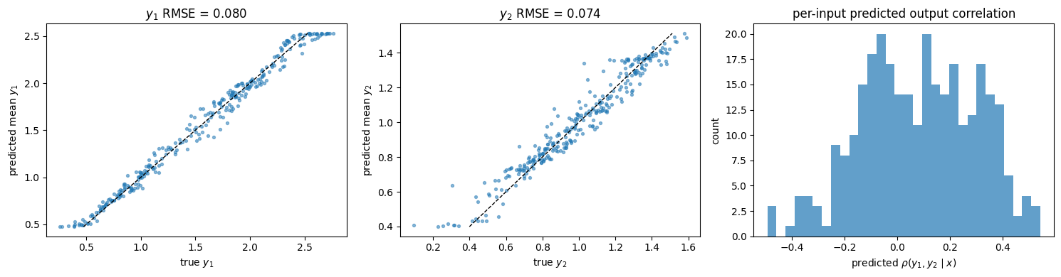
The model returns a full 2x2 predictive covariance per sample. The off-diagonal encodes the model’s belief about how \(y_1\) and \(y_2\) co-vary at that input.
Y_pred, cov_pred = model.predict_full_cov(X_te)
rho_pred = cov_pred[:, 0, 1] / np.sqrt(cov_pred[:, 0, 0] * cov_pred[:, 1, 1] + 1e-12)

fig, axes = plt.subplots(1, 3, figsize=(15, 4))
for i, (ax, ylabel) in enumerate(zip(axes[:2], ['y_1', 'y_2'])):
    ax.scatter(Yt_te[:, i], Y_pred[:, i], s=8, alpha=0.5)
    lim = [Y_pred[:, i].min(), Y_pred[:, i].max()]
    ax.plot(lim, lim, 'k--', lw=1)
    ax.set_xlabel(f'true ${ylabel}$')
    ax.set_ylabel(f'predicted mean ${ylabel}$')
    rmse = float(np.sqrt(np.mean((Y_pred[:, i] - Yt_te[:, i]) ** 2)))
    ax.set_title(f'${ylabel}$ RMSE = {rmse:.3f}')

ax = axes[2]
ax.hist(rho_pred, bins=30, color='tab:blue', alpha=0.7)
ax.set_xlabel(r'predicted $\rho(y_1, y_2 \mid x)$')
ax.set_ylabel('count')
ax.set_title('per-input predicted output correlation')
plt.tight_layout()
plt.show()
Cross-conditioning: knowing \(y_1\) tightens uncertainty on \(y_2\)
var_marg = cov_pred[:, 1, 1]
cond_mean, cond_cov, log_ev = model.predict_conditional(
    X_te, observed={0: Yt_te[:, 0]}
)
var_cond = cond_cov[:, 0, 0]
frac_kept = var_cond / np.maximum(var_marg, 1e-12)

fig, axes = plt.subplots(1, 2, figsize=(11, 4.5))
ax = axes[0]
ax.scatter(np.abs(rho_pred), 1 - frac_kept, s=10, alpha=0.5)
ax.set_xlabel(r'$|\rho_{\mathrm{pred}}(y_1, y_2 | x)|$')
ax.set_ylabel(r'$1 - \mathrm{Var}_{\mathrm{cond}} / \mathrm{Var}_{\mathrm{marg}}$')
ax.set_title('Conditioning gain vs. predicted correlation')
ax.axhline(0, color='k', lw=0.5)

ax = axes[1]
rmse_marg = float(np.sqrt(np.mean((Y_pred[:, 1] - Yt_te[:, 1]) ** 2)))
rmse_cond = float(np.sqrt(np.mean((cond_mean[:, 0] - Yt_te[:, 1]) ** 2)))
ax.bar([0, 1], [rmse_marg, rmse_cond], color=['tab:gray', 'tab:blue'])
ax.set_xticks([0, 1])
ax.set_xticklabels(['marginal\n$E[y_2|x]$', 'conditional\n$E[y_2|x, y_1]$'])
ax.set_ylabel('RMSE to true $y_2$')
ax.set_title('Conditioning sharpens point prediction too')
plt.tight_layout()
plt.show()

print(f'mean variance reduction: {(1 - frac_kept).mean():.3f}')
print(f'RMSE marginal: {rmse_marg:.3f}')
print(f'RMSE conditional: {rmse_cond:.3f}')
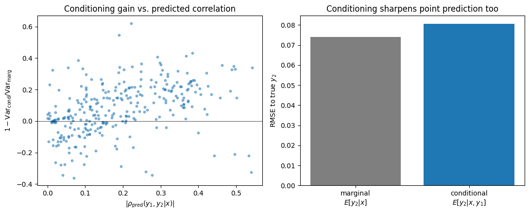
mean variance reduction: 0.078
RMSE marginal: 0.074
RMSE conditional: 0.081
Inverse design: find \(\mathbf{x}\) that produces a target \(\mathbf{y}\)
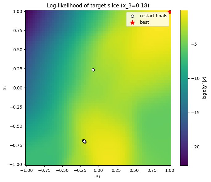
Pick a target property pair \((y_1^*, y_2^*)\) and ask: which composition \(\mathbf{x}\) should we synthesize? We optimize \(\log p(\mathbf{y}^* \mid \mathbf{x})\) by Adam ascent over \(\mathbf{x}\), with multiple random restarts to handle the multi-modal log-likelihood surface. Because the tree is fully differentiable in \(\mathbf{x}\), this is just gradient descent: no surrogate, no MCMC.
y_target = {0: 1.8, 1: 1.0}

x_best, ll_best, x_all, ll_all = model.inverse_design(
    y_target,
    n_starts=24, n_steps=600, learning_rate=0.05,
    bounds=(np.full(3, -1.0), np.full(3, 1.0)),
    random_state=0,
)

y_pred_best, std_best = model.predict(x_best.reshape(1, -1), return_std=True)
print(f'target            : y1={y_target[0]:.3f}, y2={y_target[1]:.3f}')
print(f'designed x        : {x_best.round(3)}')
print(f'predicted at best : y1={y_pred_best[0,0]:.3f} (+/-{std_best[0,0]:.3f}), '
      f'y2={y_pred_best[0,1]:.3f} (+/-{std_best[0,1]:.3f})')
print(f'log p(y* | x_best): {ll_best:.3f}')
print(f'top 5 restart log-liks: {sorted(ll_all)[-5:]}')
target            : y1=1.800, y2=1.000
designed x        : [1.    0.994 0.182]
predicted at best : y1=1.950 (+/-0.231), y2=0.955 (+/-0.159)
log p(y* | x_best): -0.056
top 5 restart log-liks: [np.float64(-0.05579432472586632), np.float64(-0.05579432472586632), np.float64(-0.05579432472586632), np.float64(-0.05579432472586632), np.float64(-0.05579432472586632)]
Visualize the design landscape
Holding \(x_3\) at the value found by inverse design, slice \(\log p(\mathbf{y}^* \mid \mathbf{x})\) over \((x_1, x_2)\) and overlay the restart finals.
import jax
import jax.numpy as jnp
from difftree._model import inverse_design_log_lik

params = model._params_jax()
obs_idx = jnp.asarray([0, 1], dtype=jnp.int32)
y_t = jnp.asarray((np.array([y_target[0], y_target[1]]) - model.y_mean_) / model.y_std_)

@jax.jit
def ll(x_std):
    return inverse_design_log_lik(
        x_std, y_t, obs_idx,
        params['W'], params['b'], params['log_gamma'],
        params['leaf_mu'], params['leaf_A'], params['leaf_chol_raw'], params['log_alpha'],
    )
ll_v = jax.vmap(ll)

x3_fixed = x_best[2]
g = np.linspace(-1.0, 1.0, 60)
X1, X2 = np.meshgrid(g, g)
Xg = np.stack([X1.ravel(), X2.ravel(), np.full(X1.size, x3_fixed)], axis=1)
Xg_std = (Xg - model.x_mean_) / model.x_std_
Lg = np.asarray(ll_v(jnp.asarray(Xg_std))).reshape(X1.shape)

fig, ax = plt.subplots(figsize=(7, 6))
im = ax.pcolormesh(X1, X2, Lg, cmap='viridis', shading='auto')
plt.colorbar(im, ax=ax, label=r'$\log p(\mathbf{y}^* | x)$')
ax.scatter(x_all[:, 0], x_all[:, 1], color='white', edgecolors='black',
           s=40, marker='o', label='restart finals')
ax.scatter([x_best[0]], [x_best[1]], color='red', s=120, marker='*', label='best')
ax.set_xlabel('$x_1$')
ax.set_ylabel('$x_2$')
ax.set_title(f'Log-likelihood of target slice (x_3={x3_fixed:.2f})')
ax.legend()
plt.tight_layout()
plt.show()
Constrained inverse design: fix \(y_1\), let \(y_2\) float
Sometimes only one property is constrained. The inverse-design API takes a partial dict.
x_best_c, ll_c, x_all_c, ll_all_c = model.inverse_design(
    {0: 1.8},
    n_starts=16, n_steps=500, learning_rate=0.05,
    bounds=(np.full(3, -1.0), np.full(3, 1.0)),
    random_state=1,
)

y_pred_c, std_c = model.predict(x_best_c.reshape(1, -1), return_std=True)
print(f'target y1={1.8:.3f} (y2 unconstrained)')
print(f'designed x: {x_best_c.round(3)}')
print(f'predicted: y1={y_pred_c[0,0]:.3f} (+/-{std_c[0,0]:.3f}),  '
      f'y2={y_pred_c[0,1]:.3f} (+/-{std_c[0,1]:.3f})')
print(f'log p(y1=1.8 | x): {ll_c:.3f}')
target y1=1.800 (y2 unconstrained)
designed x: [ 0.011 -0.307 -0.286]
predicted: y1=1.869 (+/-0.271),  y2=1.239 (+/-0.210)
log p(y1=1.8 | x): 0.311
Summary
From a single fitted tree we get:
Joint marginal predictions \(p(\mathbf{y} \mid \mathbf{x})\) with full covariance, including a per-input predicted output correlation.
Closed-form cross-conditioning \(p(y_2 \mid \mathbf{x}, y_1)\) via Schur complements on each leaf’s covariance, with leaf weights re-normalized by the marginal density of the observation. Knowing one output reduces the variance and RMSE on the other.
Differentiable inverse design: the tree’s likelihood \(\log p(\mathbf{y}^* \mid \mathbf{x})\) is end-to-end differentiable in \(\mathbf{x}\), so Adam ascent (with multi-start for multimodality) just works. Constrained variants where only a subset of outputs are targeted come for free.