Diagrams

discopt.speciation.plot builds diagrams from full equilibrium calculations, so aqueous speciation, solid fields and gas phases are mutually consistent. It needs matplotlib (pip install "discopt-speciation[plot] @ git+https://github.com/jkitchin/discopt-speciation").

Every figure on this page was made by docs/figures/make_figures.py with the code shown, using the bundled phreeqc.dat (Parkhurst and Appelo 2013). The diagrams notebook walks through the same examples in more detail.

Sweeps

import numpy as np
import matplotlib.pyplot as plt
from discopt.speciation import PhreeqcDatabase, plot

db = PhreeqcDatabase.load("phreeqc.dat")
s = db.system(["Fe", "Cl"], phases=["Fe(OH)3(a)"])
sw = plot.sweep(s, "pH", np.linspace(2, 12, 41), amounts={"Fe": 1e-3, "Cl": 3e-3}, pe=4)

fig, ax = plt.subplots(figsize=(6.5, 4))
plot.plot_sweep(sw, ["Fe+3", "FeOH+2", "Fe(OH)2+", "Fe(OH)3", "Fe(OH)4-", "Fe+2"], ax=ax, floor=1e-14)
sw.get("SI:Fe(OH)3(a)")        # any quantity along the sweep

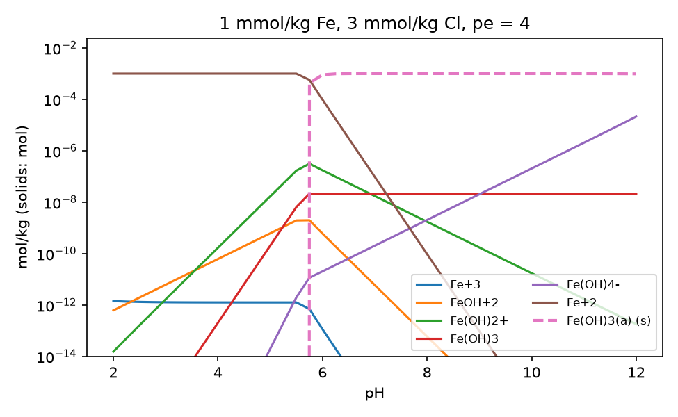
At pe 4, dissolved iron is almost all Fe²⁺ up to pH 5.5. Between pH 5.5 and 5.75 amorphous Fe(OH)₃ starts to precipitate (dashed), and by pH 6.5 it holds more than 99.6% of the iron. Each point is a full equilibrium, so the kinks where the solid appears come out of the complementarity conditions; they are not drawn in by hand.

Sweep variables. The swept variable can be:

• "pH", "pe", "T" or "P";
• an input-amount key ("Cl", "Calcite"), which gives a titration;
• "fixed:CO2(g)", a fixed log activity or partial pressure;
• a function value -> dict of equilibrate keywords, for anything else, e.g. changing two amounts together.

Solubility curves

Sweep a variable and plot a total with sw.get(fit.total(...)), or a solid amount with "solids:Gypsum". Here gypsum is heated in water with anhydrite allowed as a second phase:

from discopt.speciation import fit

cs = db.system(["Ca", "S(6)"], phases=["Gypsum", "Anhydrite"])
T = np.linspace(0, 100, 26) + 273.15
swT = plot.sweep(cs, "T", T, amounts={"Gypsum": 0.5})
dissolved_ca = fit.total("Ca+2", "CaSO4", "CaHSO4+")

fig, (a1, a2) = plt.subplots(1, 2, figsize=(9, 3.6))
a1.plot(T - 273.15, swT.get("solids:Gypsum"), label="Gypsum")
a1.plot(T - 273.15, swT.get("solids:Anhydrite"), label="Anhydrite")
a2.plot(T - 273.15, swT.get(dissolved_ca) * 1e3, "k")

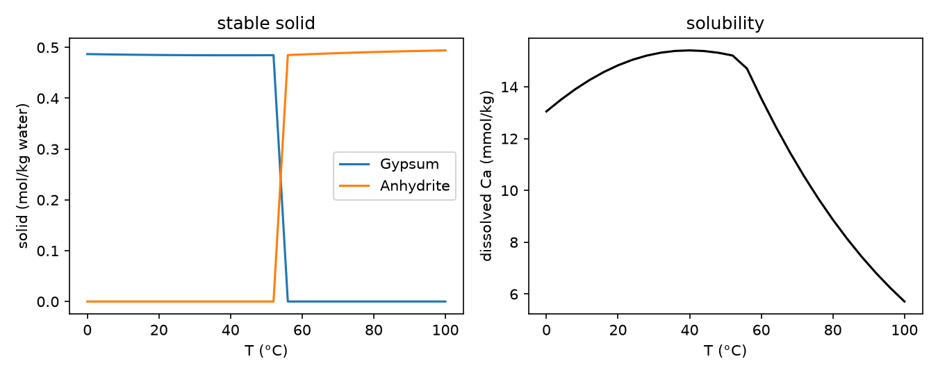
With the phreeqc.dat data, gypsum is stable up to between 52 and 56 °C (the grid spacing) and anhydrite above. Solubility follows whichever solid is stable, so the curve has a kink at the transition. No phase is selected by hand.

Predominance and Pourbaix diagrams

cands = ["Fe+2", "Fe+3", "FeOH+", "FeOH+2", "Fe(OH)2+", "Fe(OH)3", "Fe(OH)4-", "Fe(OH)3(a)"]
cands = [n for n in cands if n in s]          # keep the names this system has

fig, ax = plt.subplots(figsize=(6, 4.8))
pr, _ = plot.pourbaix(s, cands, pH=np.linspace(1, 13, 41), pe=np.linspace(-12, 20, 41),
                      amounts={"Fe": 1e-3, "Cl": 3e-3}, ax=ax)

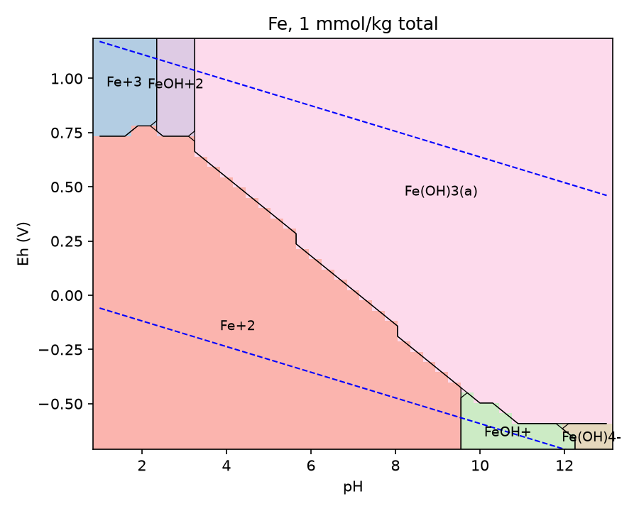
The 41 × 41 grid is 1681 equilibrium solves, about 2.5 minutes; all converged.

Classifying each point. At each grid point the candidate with the largest amount is shown: molality for aqueous species, moles for solids. Pass a dict of atom counts ({"Fe2(OH)2+4": 2, ...}) so species are compared per atom of the element of interest.

Diagram features.

• Dashed lines are the water stability limits at 1 atm.
• eh=False plots pe instead of Eh.
• pourbaix wraps predominance(system, candidates, x=(var, values), y=(var, values), **conditions), which works for any pair of variables, such as log activity–log activity or T–pH.

Cost. Each grid point is one equilibrium solve, typically 5–100 ms, so start with a coarse grid.

How this differs from classical Pourbaix diagrams. Classical diagrams (Pourbaix 1974) draw lines where two species have equal activity, for a chosen total concentration. These diagrams are computed for the stated total amounts, with activity corrections and all complexes. Boundaries move with the total concentration, which is the physically meaningful behaviour.

Ellingham diagrams

An Ellingham diagram (Ellingham 1944) plots the standard Gibbs energy of oxide formation against temperature, per mole of O₂.

R = 8.314462618e-3  # kJ/(mol K)

def from_linear(A, B):
    """log10 K(T) for dG = A + B*T in kJ per mol O2."""
    return lambda T: -(A + B * T) / (R * T * np.log(10))

oxides = {
    "2 Ni + O2 = 2 NiO": from_linear(-471.0, 0.172),
    "2 Fe + O2 = 2 FeO": from_linear(-528.0, 0.130),
    "2 H2 + O2 = 2 H2O(g)": from_linear(-492.0, 0.109),
    "C + O2 = CO2": from_linear(-394.0, -0.001),
    "2 C + O2 = 2 CO": from_linear(-223.0, -0.175),
    "4/3 Al + O2 = 2/3 Al2O3": from_linear(-1120.0, 0.214),
}
fig, ax = plt.subplots(figsize=(6.5, 4.5))
plot.ellingham(oxides, np.linspace(300, 2000, 60), per={k: 1 for k in oxides}, ax=ax)

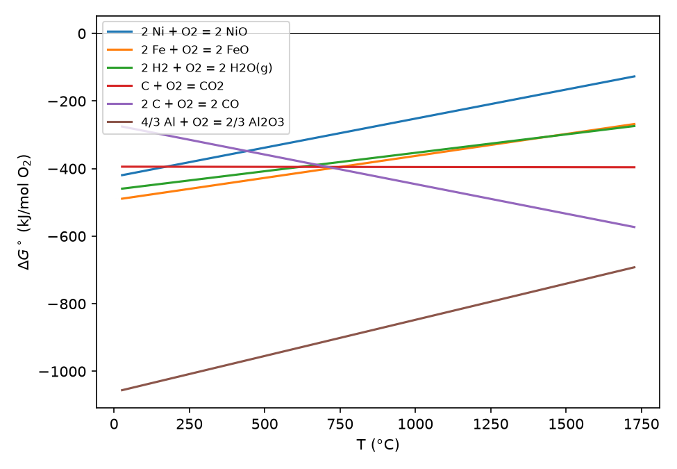
The coefficients are rounded linear fits of tabulated data, for illustration only. Lower lines are more stable oxides. The falling 2C + O₂ = 2CO line crosses FeO near 730 °C; above that, carbon reduces FeO to iron.

What is plotted. Each line is \(\Delta G^\circ(T) = -RT\ln 10\,\log K(T)\), in kJ per mol O₂ with per.

Inputs. Reactions can be Reaction objects, e.g. from a System with analytic or dH/dCp data, or plain functions T -> log10 K, e.g. from tabulated \(\Delta_f G^\circ\).

Limitation. Phase changes of metals and oxides, such as melting, appear only if your \(\log K(T)\) data include them.