Uncertainty in polynomial roots

| categories: data analysis, uncertainty | tags:

Polynomials are convenient for fitting to data. Frequently we need to derive some properties of the data from the fit, e.g. the minimum value, or the slope, etc… Since we are fitting data, there is uncertainty in the polynomial parameters, and corresponding uncertainty in any properties derived from those parameters.
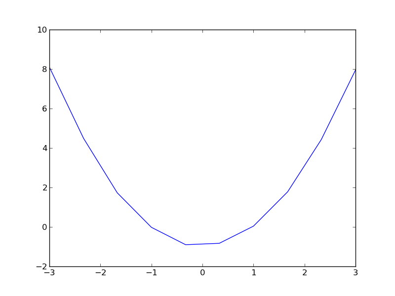
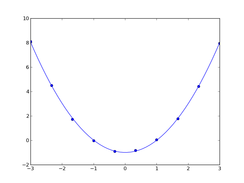
Here is our data.

-3.00 8.10
-2.33 4.49
-1.67 1.73
-1.00 -0.02
-0.33 -0.90
0.33 -0.83
1.00 0.04
1.67 1.78
2.33 4.43
3.00 7.95
import matplotlib.pyplot as plt

x = [a[0] for a in data]
y = [a[1] for a in data]
plt.plot(x, y)
plt.savefig('images/uncertain-roots.png')

import matplotlib.pyplot as plt
import numpy as np
from pycse import regress

x = np.array([a[0] for a in data])
y = [a[1] for a in data]

A = np.column_stack([x**0, x**1, x**2])

p, pint, se = regress(A, y, alpha=0.05)

print p

print pint

print se

plt.plot(x, y, 'bo ')

xfit = np.linspace(x.min(), x.max())
plt.plot(xfit, np.dot(np.column_stack([xfit**0, xfit**1, xfit**2]), p), 'b-')
plt.savefig('images/uncertain-roots-1.png')
[-0.99526746 -0.011546    1.00188999]
[[-1.05418017 -0.93635474]
 [-0.03188236  0.00879037]
 [ 0.98982737  1.01395261]]
[ 0.0249142   0.00860025  0.00510128]

Since this is a quadratic equation, we know the roots analytically: \(x = \frac{-b \pm \sqrt{b^2 - 4 a c}{2 a}\). So, we can use the uncertainties package to directly compute the uncertainties in the roots.

import numpy as np
import uncertainties as u

c, b, a = [-0.99526746, -0.011546,    1.00188999]
sc, sb, sa = [ 0.0249142,   0.00860025,  0.00510128]

A = u.ufloat((a, sa))
B = u.ufloat((b, sb))
C = u.ufloat((c, sc))

# np.sqrt does not work with uncertainity
r1 = (-B + (B**2 - 4 * A * C)**0.5) / (2 * A)
r2 = (-B - (B**2 - 4 * A * C)**0.5) / (2 * A)

print r1
print r2
1.00246826738+/-0.0134477390832
-0.990944048037+/-0.0134208013339

The minimum is also straightforward to analyze here. The derivative of the polynomial is \(2 a x + b\) and it is equal to zero at \(x = -b / (2 a)\).

import numpy as np
import uncertainties as u

c, b, a = [-0.99526746, -0.011546,    1.00188999]
sc, sb, sa = [ 0.0249142,   0.00860025,  0.00510128]

A = u.ufloat((a, sa))
B = u.ufloat((b, sb))

zero = -B / (2 * A)
print 'The minimum is at {0}.'.format(zero)
The minimum is at 0.00576210967034+/-0.00429211341136.

You can see there is uncertainty in both the roots of the original polynomial, as well as the minimum of the data. The approach here worked well because the polynomials were low order (quadratic or linear) where we know the formulas for the roots. Consequently, we can take advantage of the uncertainties module with little effort to propagate the errors. For higher order polynomials, we would probably have to do some wrapping of functions to propagate uncertainties.

Copyright (C) 2013 by John Kitchin. See the License for information about copying.

org-mode source

Discuss on Twitter

Estimating uncertainties in equations of state

| categories: uncategorized | tags:

We often use DFT to calculate the energy of a unit cell as a function of volume. Then, we fit an equation of state to the data to estimate the volume that minimizes the total energy, and the bulk modulus of the material. 10.1016/j.comphys.2003.12.001

volume energy
324.85990899 -399.9731688470
253.43999457 -400.0172393178
234.03826687 -400.0256270548
231.12159387 -400.0265690700
228.40609504 -400.0273551120
225.86490337 -400.0280030862
223.47556626 -400.0285313450
221.21992353 -400.0289534593
219.08319566 -400.0292800709
217.05369547 -400.0295224970
215.12089909 -400.0296863867
213.27525144 -400.0297809256
211.51060823 -400.0298110000
203.66743321 -400.0291665573
197.07888649 -400.0275017142
191.39717952 -400.0250998136
186.40163591 -400.0221371852
181.94435510 -400.0187369863
177.92077043 -400.0149820198
174.25380090 -400.0109367042
170.88582166 -400.0066495100
167.76711189 -400.0021478258
164.87096104 -399.9974753449
159.62553397 -399.9876885136
154.97005460 -399.9774175487
150.78475335 -399.9667603369
146.97722201 -399.9557686286
143.49380641 -399.9445262604
import numpy as np
import matplotlib.pyplot as plt
from pycse import nlinfit

# data
V = np.array([row[0] for row in data]) 
E = np.array([row[1] for row in data])

plt.plot(V, E, '.')
plt.xlabel('Volume ($\AA^3$)')
plt.ylabel('Energy (Ha)')

def Murnaghan(vol, E0, B0, BP, V0):
    '''
    given a vector of parameters and volumes, return a vector of energies.
    equation From PRB 28,5480 (1983)
    '''
    
    E = E0 + B0*vol/BP*(((V0/vol)**BP)/(BP-1)+1) - V0*B0/(BP-1.)

    return E

guess = [-400, 0.5, 2, 210]
pars, pint, SE = nlinfit(Murnaghan, V, E, guess, alpha=0.05)
E0, B0, BP, V0 = pint

Vfit = np.linspace(V.min(), V.max())
plt.plot(Vfit, Murnaghan(Vfit, *pars))
plt.savefig('images/eos-uncertainty.png')

print '95% confidence intervals'
print 'V0 = {0} bohr**3'.format(V0)
print 'E0 = {0} Ha'.format(E0)
print 'B0 = {0} GPA'.format([x * 29421.010901602753 for x in B0])
95% confidence intervals
V0 = [212.27788154532402, 213.27897592511891] bohr**3
E0 = [-400.0297027767362, -400.02922937100408] Ha
B0 = [108.62283904402159, 111.20447706313001] GPA

You can see the fit is not perfect, and there is corresponding uncertainty in the estimated parameters. A nice feature of the Murnaghan equation of state is that the parameters are directly the quantities of interest, so the uncertainties are directly calculated here. For other models, e.g. a polynomial fit, you would have to propagate the errors in the parameters to the properties.

Copyright (C) 2013 by John Kitchin. See the License for information about copying.

org-mode source

Discuss on Twitter

Estimating where two functions intersect using data

| categories: data analysis | tags:

Suppose we have two functions described by this data:

T(K) E1 E2
300 -208 -218
400 -212 -221
500 -215 -220
600 -218 -222
700 -220 -222
800 -223 -224
900 -227 -225
1000 -229 -227
1100 -233 -228
1200 -235 -227
1300 -240 -229

We want to determine the temperature at which they intersect, and more importantly what the uncertainty on the intersection is. There is noise in the data, which means there is uncertainty in any function that could be fit to it, and that uncertainty would propagate to the intersection. Let us examine the data.

import matplotlib.pyplot as plt

T = [x[0] for x in data]
E1 = [x[1] for x in data]
E2 = [x[2] for x in data]

plt.plot(T, E1, T, E2)
plt.legend(['E1', 'E2'])
plt.savefig('images/intersection-0.png')

Our strategy is going to be to fit functions to each data set, and get the confidence intervals on the parameters of the fit. Then, we will solve the equations to find where they are equal to each other and propagate the uncertainties in the parameters to the answer.

These functions look approximately linear, so we will fit lines to each function. We use the regress function in pycse to get the uncertainties on the fits. Then, we use the uncertainties package to propagate the uncertainties in the analytical solution to the intersection of two lines.

import numpy as np
from pycse import regress
import matplotlib.pyplot as plt
import uncertainties as u

T = np.array([x[0] for x in data])
E1 = np.array([x[1] for x in data])
E2 = np.array([x[2] for x in data])

# columns of the x-values for a line: constant, T
A = np.column_stack([T**0, T])

p1, pint1, se1 = regress(A, E1, alpha=0.05)

p2, pint2, se2 = regress(A, E2, alpha=0.05)

# Now we have two lines: y1 = m1*T + b1 and y2 = m2*T + b2
# they intersect at m1*T + b1 = m2*T + b2
# or at T = (b2 - b1) / (m1 - m2)
b1 = u.ufloat((p1[0], se1[0]))
m1 = u.ufloat((p1[1], se1[1]))

b2 = u.ufloat((p2[0], se2[0]))
m2 = u.ufloat((p2[1], se2[1]))

T_intersection = (b2 - b1) / (m1 - m2)
print T_intersection

# plot the data, the fits and the intersection and \pm 2 \sigma.
plt.plot(T, E1, 'bo ', label='E1')
plt.plot(T, np.dot(A,p1), 'b-')
plt.plot(T, E2, 'ro ', label='E2')
plt.plot(T, np.dot(A,p2), 'r-')

plt.plot(T_intersection.nominal_value,
        (b1 + m1*T_intersection).nominal_value, 'go',
        ms=13, alpha=0.2, label='Intersection')
plt.plot([T_intersection.nominal_value - 2*T_intersection.std_dev(),
          T_intersection.nominal_value + 2*T_intersection.std_dev()],
         [(b1 + m1*T_intersection).nominal_value, 
          (b1 + m1*T_intersection).nominal_value],
         'g-', lw=3, label='$\pm 2 \sigma$')
       
plt.legend(loc='best')
plt.savefig('images/intersection-1.png')
813.698630137+/-62.407180552

You can see there is a substantial uncertainty in the temperature at approximately the 90% confidence level (± 2 σ).

Update 7-7-2013

After a suggestion from Prateek, here we subtract the two data sets, fit a line to that data, and then use fsolve to find the zero. We wrap fsolve in the uncertainties package to directly get the uncertainty on the root.

import numpy as np
from pycse import regress
import matplotlib.pyplot as plt
import uncertainties as u
from scipy.optimize import fsolve


T = np.array([x[0] for x in data])
E1 = np.array([x[1] for x in data])
E2 = np.array([x[2] for x in data])

E = E1 - E2

# columns of the x-values for a line: constant, T
A = np.column_stack([T**0, T])

p, pint, se = regress(A, E, alpha=0.05)

b = u.ufloat((p[0], se[0]))
m = u.ufloat((p[1], se[1]))

@u.wrap
def f(b, m):
    X, = fsolve(lambda x: b + m * x, 800)
    return X

print f(b, m)
813.698630137+/-54.0386903923

Interesting that this uncertainty is a little smaller than the previously computed uncertainty. Here you can see we have to wrap the function in a peculiar way. The function must return a single float number, and take arguments with uncertainty. We define the polynomial fit (a line in this case) in a lambda function inside the function. It works ok.

Copyright (C) 2013 by John Kitchin. See the License for information about copying.

org-mode source

Discuss on Twitter

Memoizing instance methods in a class

| categories: programming | tags:

Suppose you have a module that you import a class from, and the class defines some methods that you want to memoize. You do not want to modify the source code, maybe because it is not your code, or because you do not want to maintain it, etc… Here is one way to modify the class functions at runtime. We will use the memoize decorator and replace the class function definition with the wrapped function that caches the results. We also allow arbitrary arguments and keyword arguments. A subtle wrinkle here is that you cannot use a dictionary as a key to a dictionary because dictionaries are not hashable. We use the pickle module to created a string that should uniquely represent the args and keyword args, and we use that string as the key.

class Calculator:
    def __init__(self):
        pass

    def calculate(self, a):
        'returns the answer to everything'
        return 42

    def method_2(self, *args, **kwargs):
        return (args, kwargs)


import pickle

from functools import wraps
def memoize(func):
    cache = {}
    @wraps(func)
    def wrap(*args,**kwargs):
        key = pickle.dumps((args, kwargs))
        if key not in cache:
            print 'Running func with ', args
            cache[key] = func(*args, **kwargs)
        else:
            print 'result in cache'
        return cache[key]
    return wrap

# now monkey patch/decorate the class function
Calculator.calculate = memoize(Calculator.calculate)
Calculator.method_2 = memoize(Calculator.method_2)

calc = Calculator()
print calc.calculate(3)
print calc.calculate(4)
print calc.calculate(3)


print calc.method_2()

print calc.method_2(1,2)

print calc.method_2(1,2,a=5)
Running func with  (<__main__.Calculator instance at 0x0000000001E9B3C8>, 3)
42
result in cache
42
Running func with  (<__main__.Calculator instance at 0x0000000001E9B3C8>, 4)
42
result in cache
42
Running func with  (<__main__.Calculator instance at 0x0000000001E9B3C8>,)
((), {})
result in cache
((), {})
Running func with  (<__main__.Calculator instance at 0x0000000001E9B3C8>, 1, 2)
((1, 2), {})
result in cache
((1, 2), {})
Running func with  (<__main__.Calculator instance at 0x0000000001E9B3C8>, 1, 2)
((1, 2), {'a': 5})
result in cache
((1, 2), {'a': 5})

This particular memoize decorator is not persistent; the data is only stored in memory. You would have to write the data out to a file and reread the file to make it persistent.

It is not obvious this practice is good; you have in essence changed the behavior of the original function in a way that may be hard to debug, and could conceivably be incompatible with the documentation of the function.

An alternative approach is writing another function that wraps the code you want, and memoize that function.

class Calculator:
    def __init__(self):
        pass

    def calculate(self, a):
        'returns the answer to everything'
        return 42


from functools import wraps
def memoize(func):
    cache = {}
    @wraps(func)
    def wrap(*args):
        if args not in cache:
            print 'Running func with ', args
            cache[args] = func(*args)
        else:
            print 'result in cache'
        return cache[args]
    return wrap

calc = Calculator()

@memoize
def my_calculate(a):
    return calc.calculate(a)

print my_calculate(3)
print my_calculate(4)
print my_calculate(3)
Running func with  (3,)
42
result in cache
42
Running func with  (4,)
42
result in cache
42

It is debatable whether this is cleaner. One argument for this is that it does not monkey with the original code at all.

Copyright (C) 2013 by John Kitchin. See the License for information about copying.

org-mode source

Discuss on Twitter

New paper accepted on CO_2 capture simulation

| categories: news | tags:

Our manuscript titled "Comparisons of Amine Solvents for Post-combustion CO\(_2\) Capture: A Multi-objective Analysis Approach" by Anita Lee, John Eslick, David Miller, and John Kitchin was just accepted in International Journal of Greenhouse Gas Control. In this paper we used a genetic algorithm to find pareto-optimal operating conditions of amine solvent CO2 capture systems that minimize capital cost and parasitic power cost. We compared MEA, DEA and AMP, and found that there are operating conditions where both solvents could be better than MEA.

Update: The article is online here: http://www.sciencedirect.com/science/article/pii/S1750583613002703

Copyright (C) 2013 by John Kitchin. See the License for information about copying.

org-mode source

Discuss on Twitter
« Previous Page -- Next Page »