Add subheadings to all headings in an org-file at some level

| categories: org-mode | tags:

On the org-mode mailing list someone asked how to insert a sub-heading with properties at some level in a tree. The application is they have a tree they use to store grades for a class, and they want to easily add a new level for an assignment for each student. The new level will have a title, and some properties to store the grade in.

This can be done with org-map-entries. This will visit all the headlines and run a function. For this example, students are at level 3, and we want to add a headline at level 4 with the title "Essay 2", and with a property for the grade. The following code does this.

(let ((MATCH t)
      (SCOPE 'file)
      (SKIP nil)
      (spacing nil))
  (org-map-entries
             (lambda ()
               (let ((level (nth 1 (org-heading-components))))
                 (if (= level 3)                     
                     (save-restriction
                       (org-narrow-to-subtree)
                       (goto-char (point-max))
                       
                       (org-insert-heading)
                       (insert "Essay 2\n")
                       (org-entry-put (point) "GRADE" nil)
                       ;; now cut tree and paste at level 4
                       (org-cut-subtree)
                       (org-paste-subtree 4)
                       )))) MATCH SCOPE SKIP))

This code does not check for duplicates, so if you run it again, you get another set of entries for Essay 2. That might actually be hard to prevent without setting a unique ID for each new entry, something like Student-Name-Essay-2.

I found it necessary to cut and paste the new subtree to get to the level I wanted because in Class two, there were not already subtrees at level 4, and the code above went into a recursion loop.

I could not figure out why I had to narrow to the subtree, and go to the end of that subtree. Without doing that there was another recursion loop.

Below here is a slightly modified subtree showing a structure of two courses an instructor might have, with students in headlines at level 3. The code above has already added headlines at level 4 for "Essay 2". You have to check out the actual org-file to see that the properties are there.

For application, the code above could be put in an emacs-lisp file as an interactive command you could call with M-x.

1 Class One

1.1 Student 1

1.1.1 Essay One

Here is my comment to the student on their essay. The grade/mark itself will be stored as a property or priority. <<<<<<<<<<<<<<HERE I'd like to add a node for "Essay Two"

1.1.2 Essay 2

1.2 Student 2

Comment on John's essay. <<<<<<<<<<<<<< I to add the same node skeleton here, automatically

1.2.1 Essay 2

1.3 Student 3

1.3.1 Essay One

Comment on Sally's essay. <<<<<<<<<<<<<< And here.

1.3.2 Essay 2

2 Class Two

2.1 Student 1

2.1.1 Essay 2

2.2 Student 2

2.2.1 Essay 2

Copyright (C) 2013 by John Kitchin. See the License for information about copying.
org-mode source

Discuss on Twitter

Git archives for data sharing

| categories: data | tags:

in some past posts we have looked at constructing JSON files for data sharing. While functional, that approach requires some extra work to create the data files for sharing, and may not be useful for all sorts of data. For instance you may not want to store electron density in a JSON file.

Here we consider using git archives for packaging exactly the data you used in the same hierarchy as on your file system. The idea is to store your work in a git repository. You commit any data files you would want to share, and then create an archive of that data. This enables you to control what gets shared, while keeping the data that should not be shared out of the archive.

We will run a few VASP calculations, and summarize each one in a JSON file. We will commit those JSON files to the git repository, and finally make a small archive that contains them.

1 A molecule

Calculate the total energy of a CO molecule.

from ase import Atoms, Atom
from jasp import *
import numpy as np
import json
np.set_printoptions(precision=3, suppress=True)

co = Atoms([Atom('C',[0,   0, 0]),
            Atom('O',[1.2, 0, 0])],
            cell=(6., 6., 6.))

with jasp('molecules/simple-co', #output dir
          xc='PBE',  # the exchange-correlation functional
          nbands=6,  # number of bands
          encut=350, # planewave cutoff
          ismear=1,  # Methfessel-Paxton smearing
          sigma=0.01,# very small smearing factor for a molecule
          atoms=co) as calc:
    print 'energy = {0} eV'.format(co.get_potential_energy())
    print co.get_forces()
    with open('JSON', 'wb') as f:
        f.write(json.dumps(calc.dict))
    os.system('git add JSON')
energy = -14.687906 eV
[[ 5.095  0.     0.   ]
 [-5.095  0.     0.   ]]

2 A bulk calculation

Now we run a bulk calculation

from jasp import *

from ase import Atom, Atoms

atoms = Atoms([Atom('Cu',  [0.000,      0.000,      0.000])],
              cell=  [[ 1.818,  0.000,  1.818],
                      [ 1.818,  1.818,  0.000],
                      [ 0.000,  1.818,  1.818]])

with jasp('bulk/alloy/cu',
          xc='PBE',
          encut=350,
          kpts=(13,13,13),
          nbands=9,
          ibrion=2,
          isif=4,
          nsw=10,
          atoms=atoms) as calc:
    print atoms.get_potential_energy()
    with open('JSON', 'wb') as f:
        f.write(json.dumps(calc.dict))
    os.system('git add JSON')
-3.723306

3 Analysis via the JSON files

This analysis is independent of jasp and therefore is portable

We can retrieve the bulk data

import json

with open('bulk/alloy/cu/JSON', 'rb') as f:
    d = json.loads(f.read())
    print d['data']['total_energy']
-3.723306

Or the molecule data:

import json

with open('molecules/simple-co/JSON', 'rb') as f:
    d = json.loads(f.read())
    print d['data']['total_energy']
-14.687906

4 Create the archive file

As you do your work, you add and commit files as needed. For this project all that needs to be shared are the JSON files, and the scripts (which are in this document) that we used to run the calculations and do the analysis. If we are satisfied with the state of the git repository, we create an archive like this:

git archive --format zip HEAD -o archive.zip

Here is the result: archive.zip .

You can download the zip file, unzip it, and rerun the analysis to extract the total energies on any system with a modern Python installation.

5 Summary

This seems to be an easy way to share data from a single project, i.e. a single git repository. It isn't obvious how you would package data from multiple projects, or how you would run multiple projects in a single directory.

Copyright (C) 2013 by John Kitchin. See the License for information about copying.

org-mode source

Discuss on Twitter

Hatched symbols in matplotlib

| categories: plotting | tags:

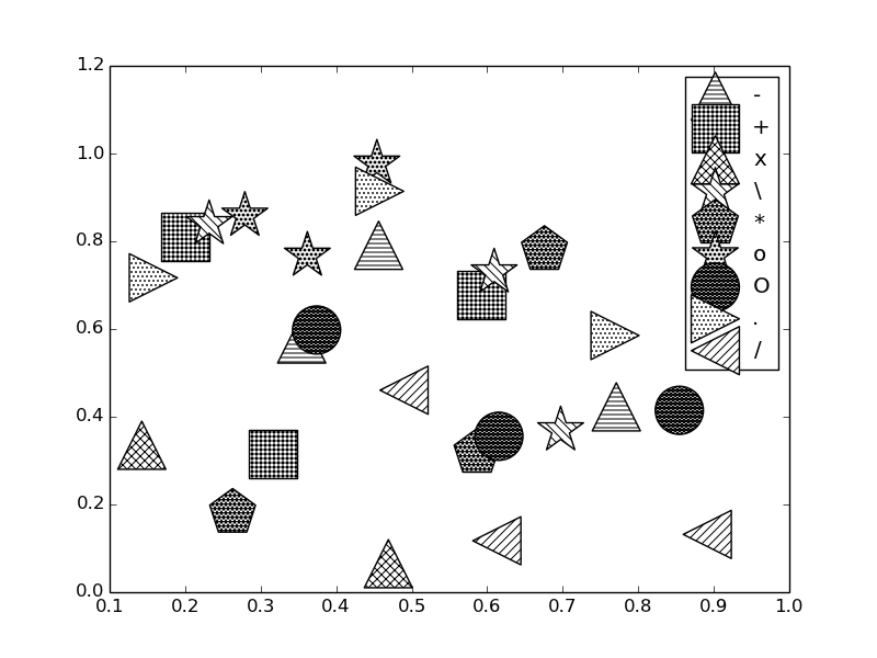
I learned something new about matplotlib today: How to make hatched (patterned) symbols in a plot. Well, sort of. The scatter plot in matplotlib has a hatch keyword argument that specifies a pattern on the marker. Below, is an example that runs through a handful of hatch patterns, on randomly selected symbols.

Curiously, hatch is not a kwarg of the scatter function, but of collections . Anyway, let us see how to get the hatched symbols.

import random
import numpy as np
import matplotlib.pyplot as plt

patterns = ('-', '+', 'x', '\\', '*', 'o', 'O', '.', '/')
markers = 'os<^>p*'
for pattern in patterns:
    plt.scatter(np.random.uniform(size=(3,1)), np.random.uniform(size=(3,1)), s=1000,
                marker=random.choice(markers),
                facecolor='white',
                hatch=3*pattern, label=pattern)

plt.legend(scatterpoints=1, loc='best')
plt.savefig('images/hatched-symbols.png')

There are some other interesting things you can do with filled markers , hatched contours and with hatched bar graphs . Note this hatching is specific to plt.scatter. It does not work with plt.plot.

Copyright (C) 2013 by John Kitchin. See the License for information about copying.

org-mode source

Discuss on Twitter

Writing exams in org-mode

| categories: org-mode | tags:

There are a few aspects of writing exams that are tedious the way I normally do it. Typically I write exams in Word because I can easily see the layout, how much whitespace there is to write answers in, etc… I like to put a gradesheet on the final page which lists each problem, the points it is worth, and a blank to put the grade for that problem into. It is tedious to go back through 10 pages of questions to look up all the points, enter them in, add them up, etc… And if I decide to renumber the questions or move them, it must be repeated.

Construction of the grade sheet ought to be automated. That is not going to happen in my hands in MS Word. I have seen this done in LaTeX in the Acrotex educational package, but I don't see myself hacking LaTeX any time soon either. Enter org-mode. I could see writing the exam in org-mode, and writing some code to construct the grade table.

The idea is that we would store the points in a PROPERTY of an org-heading. Then, to create the table, we just loop through the headlines, gather the levels and points, and then construct a table to put in the exported LaTeX. The next section contains some exam questions that will form the basis of this post.

1 The exam section

1.1 Do you get it?

What is the answer to the universe? \vspace{2cm}

1.2 Multipart question

1.2.1 Circle the best answer

What is 1 + 1? a) 2 b) 3 c) 4

1.2.2 Describe a cat.

\vspace{2cm}

1.3 Essay question

Expound on the meaning of life. \vspace{3cm}

2 Back to the grade table construction

We will parse the buffer to get the headlines, and then extract some properties from each headline. For each headline that has points we will print the title and points it is worth, and finally the total number of points.

(setq total-points 0)    ; counter for the total points

;; now loop over headlines
(org-element-map 
    (org-element-parse-buffer 'headline) 'headline 
  ;; function to print headline title and points
  (lambda (headline) 
    (let ((points (org-element-property :POINTS headline))
          (title  (org-element-property :title headline)))
      (if points (progn
                   (setq total-points (+ total-points (string-to-number points)))
                   (princ (format "title=%s\nPOINTS=%s\n\n" title points)))))))

(princ (format "Total points = %s" total-points))
title=Do you get it?
POINTS=5

title=Circle the best answer
POINTS=10

title=Describe a cat.
POINTS=4

title=Essay question
POINTS=25

Total points = 44

That is the foundation for the grade table. What I would like is the grade table to be structured like this:

problem Points grade
ref to heading #points  

Where the ref to heading is the same number as the actual heading. During the export, labels are generated for each section, which we could refer to. To take advantage of this we need to figure out what the labels are, so we can refer to them.

After quite a bit of hackery, I figured out how to access this information 1. It is not readily apparent this is how to do it, but it works!

(let* ((info (org-export-collect-tree-properties (org-element-parse-buffer 'headline) '()))
       (headline-numbering (plist-get info :headline-numbering)))
(org-element-map (plist-get info :parse-tree) 'headline
  (lambda (headline) 
    (format "\\ref{sec-%s}" (mapconcat 
                      (lambda (x) (format "%s" x)) (cdr (assoc headline headline-numbering)) "-")))))
("\\ref{sec-1}" "\\ref{sec-2}" "\\ref{sec-2-1}" "\\ref{sec-2-2}" "\\ref{sec-2-2-1}" "\\ref{sec-2-2-2}" "\\ref{sec-2-3}" "\\ref{sec-3}" "\\ref{sec-}")

So, let us try putting this all together 2.

(setq total-points 0)    ; counter for the total points
(princ "#+caption: The grade table\n")
(princ "#+attr_latex: :align |c|c|c|\n")
(princ "|-\n")
(princ "|Problem|Possible Points|Points earned|\n|-\n")
(let* ((info (org-export-collect-tree-properties (org-element-parse-buffer 'headline) '()))
       (headline-numbering (plist-get info :headline-numbering)))
  (org-element-map (plist-get info :parse-tree) 'headline
    (lambda (headline) 
      (let ((ref (format "\\ref{sec-%s}" (mapconcat 
                                          (lambda (x) (format "%s" x)) (cdr (assoc headline headline-numbering)) "-")))
            (points (org-element-property :POINTS headline)))
        (if points (progn
                     (setq total-points (+ total-points (string-to-number points)))
                     (princ (format "|%s|%s|  |\n|-\n" ref points))))))))

(princ (format "| |Total points| %s|\n" total-points))
(princ "|-\n")
Table 1: The grade table
Problem Possible Points Points earned
\ref{sec-1-1-1} 5  
\ref{sec-1-1-2-1} 10  
\ref{sec-1-1-2-2} 4  
\ref{sec-1-1-3} 25  
  Total points 44

Note this table gets munged by Mathjax in HTML. I am not sure that is fixable. You can open the pdf and see the results.

This works ok. There is still some work to be done. For example the boxes in the grade table are not very large. The references are a little odd in this case, but that is an artifact of the fact that you cannot nest a section deeper than 3 levels in LaTeX without some work, and I nested my exam section in a second level heading so it would appear in the blog post. A real application of this would not have all these other sections, and would not export the build section. It is a tad tedious to hand build the table, but not too bad.

It might be better to use CUSTOM_ID labels in the sections, rather than try to build up the references. You still need to think about what the labels would be, and we are used to seeing numbers!

3 building the pdf

I have gotten in the habit of building the latex file from commands, and manually running them with C-c C-c.

(let ((org-latex-default-packages-alist
       '(("" "minted" nil)
         ("linktocpage,
  pdfstartview=FitH,
  colorlinks,
  linkcolor=blue,
  anchorcolor=blue,
  citecolor=blue,
  filecolor=blue,
  menucolor=blue,
  urlcolor=blue" "hyperref" t)))
      (async nil)
      (subtreep nil)
      (visible-only nil)
      (body-only nil))

  (org-latex-export-to-latex async subtreep visible-only body-only '()))
(progn
  (shell-command "pdflatex -shell-escape writing-exams-in-orgmode")
  (shell-command "pdflatex -shell-escape writing-exams-in-orgmode"))

Footnotes:

1

This code does not generate correct labels for headlines with TODO in them, or for footnotes.

2

Note this table gets munged by Mathjax in HTML.

Copyright (C) 2013 by John Kitchin. See the License for information about copying.

org-mode source

Discuss on Twitter

Sharing data via JSON files

| categories: ase, dft | tags:

Table of Contents

In a previous post I discussed how to represent a single DFT calculation in a JSON file that could easily be shared, and reanalyzed. Here I look at sharing a series of calculations. I had previously run calculations to analyze an equation of state for Cu. Here we create a list of the JSON representations of each calculation, and save it in one overall JSON file. We will give the data some structure and documentation. JSON represents dictionaries very well, so we build a dictionary of the results and then "dump" that dictionary to a JSON file.

from jasp import *

LC = [3.5, 3.55, 3.6, 3.65, 3.7, 3.75]

data = {'doc':'JSON file containing a set of calculations for the equation of state of Cu'}

data['calculations'] = []

for a in LC:
    with jasp('../bulk/Cu-{0}'.format(a)) as calc:
        data['calculations'].append(calc.dict)

import json
with open('eos.json', 'wb') as f:
    f.write(json.dumps(data))

Now, you can view this eos.json file, and analyze it yourself as follows. In python we read the file in and convert it to a data structure using the json module.

import json

with open('eos.json', 'rb') as f:
    d = json.loads(f.read())

volumes =  [entry['data']['volume'] for entry in d['calculations']]
energies = [entry['data']['total_energy'] for entry in d['calculations']]

import matplotlib.pyplot as plt
plt.plot(volumes, energies)
plt.xlabel('Volume ($\AA$)')
plt.ylabel('Total energy (eV)')
plt.savefig('eos-from-json.png')
plt.show()

If you wanted to do further analysis you could. Suppose you wanted to know more detail about how that calculation was done? You can retrieve the INCAR, KPOINT, and POTCAR details for each calculation. Any parameter not listed here was not specified in the calculations.

import json

with open('eos.json', 'rb') as f:
    d = json.loads(f.read())

# print details for the first calculation in the list
print d['calculations'][0]['incar']
print d['calculations'][0]['input']
print d['calculations'][0]['potcar']
{u'doc': u'INCAR parameters', u'nbands': 9, u'encut': 350.0, u'prec': u'Normal'}
{u'kpts': [8, 8, 8], u'reciprocal': False, u'xc': u'PBE', u'kpts_nintersections': None, u'setups': None, u'txt': u'-', u'gamma': False}
[[u'Cu', u'potpaw_PBE/Cu/POTCAR', u'a44c591415026f53deb16a99ca3f06b1e69be10b']]

The POTCAR information contains the species, the path to the POTCAR, and a git-hash of the POTCAR file. That way you can tell if you used exactly the same file that I did. You can compute a git hash like this :

cat /home-research/jkitchin/src/vasp/potpaw_PBE/Cu/POTCAR | git hash-object --stdin
a44c591415026f53deb16a99ca3f06b1e69be10b

If you want to get the details of the geometry of some calculation, you do it this way:

import json

with open('eos.json', 'rb') as f:
    d = json.loads(f.read())

print d['calculations'][0]['atoms'].keys()
print 'cell = ', d['calculations'][0]['atoms']['cell']
print 'syms = ', d['calculations'][0]['atoms']['symbols']
print 'cpos = ', d['calculations'][0]['atoms']['positions']
[u'cell', u'symbols', u'positions', u'pbc', u'tags']
cell =  [[1.75, 1.75, 0.0], [0.0, 1.75, 1.75], [1.75, 0.0, 1.75]]
syms =  [u'Cu']
cpos =  [[0.0, 0.0, 0.0]]

You can do further analysis from there.

1 Summary

This looks ok as a data sharing mechanism. The json file here is pretty small (6.8 kb), and pretty easy to work with. Clearly some thought must go into how the data is structured so you know what to get, and how you get it. That could even be documented in the json file itself. For instance, each calculator has a doc element that describes what is in it. The json file we made above also has that data.

import json

with open('eos.json', 'rb') as f:
    d = json.loads(f.read())

print d['doc']
print
print d['calculations'][0]['doc']
JSON file containing a set of calculations for the equation of state of Cu

JSON representation of a VASP calculation.

energy is in eV
forces are in eV/\AA
stress is in GPa (sxx, syy, szz,  syz, sxz, sxy)
magnetic moments are in Bohr-magneton
The density of states is reported with E_f at 0 eV.
Volume is reported in \AA^3
Coordinates and cell parameters are reported in \AA

If atom-projected dos are included they are in the form:
{ados:{energy:data, {atom index: {orbital : dos}}}

For archival purposes you may want to put a creation date, contact data, etc… in the file too.

Copyright (C) 2013 by John Kitchin. See the License for information about copying.

org-mode source

Discuss on Twitter
« Previous Page -- Next Page »