New publication - Spin-informed universal graph neural networks for simulating magnetic ordering

| categories: publication, news | tags:

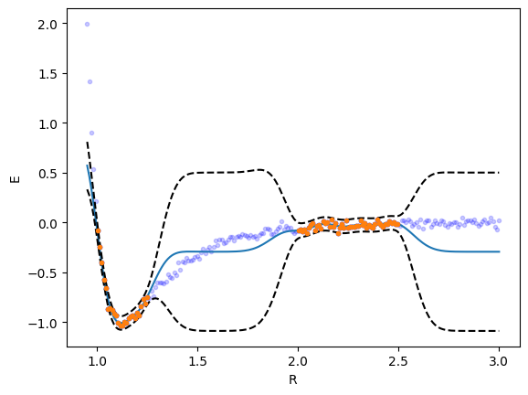
In this work, we developed a data-efficient, spin-informed graph neural network framework that augments universal machine-learning interatomic potentials with explicit spin coordinates and initial magnetic-moment guesses, while rigorously preserving the physical symmetries of collinear magnetism. This allows us to predict both the magnitude and direction of atomic spins in bulk and surface materials. By integrating a closed-loop anomaly detection pipeline based on Gaussian mixture models and z-score outlier filtering, we uncovered and corrected mislabeled DFT data, substantially improving dataset quality and model robustness. The resulting SI-GemNet-OC model achieves state-of-the-art accuracy, dramatically speeds up DFT convergence (e.g., reducing SCF cycles for GdDyAl₄ from 211 to 28), and successfully ranks magnetic orderings across hundreds of compounds with a Spearman’s ρ of 0.896. Importantly, we also show that this approach generalizes to complex surface and adsorbate-induced spin configurations, offering a powerful new tool for high-throughput discovery of magnetic materials.

@article{xu-2025-spin-infor,
  author =       {Wenbin Xu and Rohan Yuri Sanspeur and Adeesh Kolluru and Bowen
                  Deng and Peter Harrington and Steven Farrell and Karsten
                  Reuter and John R. Kitchin },
  title =        {Spin-Informed Universal Graph Neural Networks for Simulating
                  Magnetic Ordering},
  journal =      {Proceedings of the National Academy of Sciences},
  volume =       122,
  number =       27,
  pages =        {e2422973122},
  year =         2025,
  doi =          {10.1073/pnas.2422973122},
  URL =          {https://www.pnas.org/doi/abs/10.1073/pnas.2422973122},
  eprint =       {https://www.pnas.org/doi/pdf/10.1073/pnas.2422973122},
}

Copyright (C) 2025 by John Kitchin. See the License for information about copying.

org-mode source

Org-mode version = 9.8-pre

Discuss on Twitter

New publication - Hyperplane decision trees as piecewise linear surrogate models for chemical process design

| categories: publication, news | tags:

We’ve developed a new kind of decision-tree model that’s both smart and practical for tackling tough engineering problems. First, we take raw data and "lift" it into a richer feature space so we can slice it more cleverly including angular shapes. Next, we grow a friendly “hyperplane” tree that splits data along these angled cuts, fitting simple linear models in each branch. The result is a piecewise-linear surrogate that behaves a lot like the real system but runs orders of magnitude faster. Finally, because each piece is just a linear model, we can plug the whole thing straight into an optimizer that finds the very best solution under complex rules. That means we can design chemical processes, heat exchangers, or any engineering system more reliably and sustainably - saving time, energy, and cost.

@article{sunshine-2025-hyper-decis,
  author =       {Ethan M. Sunshine and Carolina Colombo Tedesco and Sneha A.
                  Akhade and Matthew J. McNenly and John R. Kitchin and Carl D.
                  Laird},
  title =        {Hyperplane Decision Trees As Piecewise Linear Surrogate Models
                  for Chemical Process Design},
  journal =      {Computers \& Chemical Engineering},
  volume =       {},
  number =       {},
  pages =        109204,
  year =         2025,
  doi =          {10.1016/j.compchemeng.2025.109204},
  url =          {https://doi.org/10.1016/j.compchemeng.2025.109204},
  DATE_ADDED =   {Wed Jul 9 14:14:17 2025},
}

Copyright (C) 2025 by John Kitchin. See the License for information about copying.

org-mode source

Org-mode version = 9.8-pre

Discuss on Twitter

Lies, damn lies, statistics and Bayesian statistics

| categories: machine-learning | tags:

This post on LinkedIn (https://www.linkedin.com/posts/activity-7341134401705041920-gaEd?utm_source=share&utm_medium=member_desktop&rcm=ACoAAAfqmO0BzyXpJw8w7yyHwkoMSiaKfGg-sKI) reminded me of a quip I often make of "Lies, damn lies, statistics, and Bayesian statistics". I am frequently skeptical of claims about "Bayesian something something", especially when the claim is about uncertainty quantification. That skepticism comes from practical experience of mine that "Bayesian something something" is rarely as well behaved and informative as advertised (in my hands of course).

To illustrate, I will use some noisy, 1d data from a Lennard-Jones function and Gaussian process regression to fit the data.

1. The data

We get our data by sampling a Lennard-Jones function, adding some noise, and removing a gap in the data. The gap in the middle might be classically considered an interpolation region.

import numpy as np
import matplotlib.pyplot as plt

r = np.linspace(0.95, 3, 200)

eps, sig = 1, 1
y = 4 * eps * ((1 / r)**12 - (1 / r)**6) + np.random.normal(0, 0.03, size=r.shape)


ind = ((r > 1) & (r < 1.25)) | ((r > 2) & (r < 2.5))
_R = r[ind][:, None]
_y = y[ind]
plt.plot(_R, _y, '.')
plt.xlabel('R')
plt.ylabel('E');

2. GPR with a RBF kernel

The RBF kernel is the most standard kernel. It does an ok job fitting here, although I see evidence of overfitting (the wiggles are caused by the noise). You can reduce the overfitting by using a larger alpha value in the gpr, but that requires you to know in advance how smooth it should be.

from sklearn.gaussian_process import GaussianProcessRegressor
from sklearn.gaussian_process.kernels import RBF, WhiteKernel
kernel = RBF() + WhiteKernel()
gpr = GaussianProcessRegressor(kernel=kernel,
                               random_state=0, normalize_y=True).fit(_R, _y)

plt.plot(_R, _y, 'b.')
plt.plot(r, y, 'b.', alpha=0.2)

yp, se = gpr.predict(r[:, None], return_std=True)
plt.plot(r, yp)
plt.plot(r, yp + 2 * se, 'k--', r, yp - 2 * se, 'k--');
plt.plot(_R, _y, '.')
plt.xlabel('R')
plt.ylabel('E');

gpr.kernel_
RBF(length_scale=0.0948) + WhiteKernel(noise_level=0.00635)

The uncertainty here is primarily related to the model, i.e. it is constrained to be correct where there is data, but with no data, the model is not the right one.

The model does well in the region where there is data, but is qualitatively wrong in the gap (even though classically this would be considered interpolation), and overestimates the uncertainty in this region. The problem is the covariance kernel decays to 0 about two length scales away from the last point, which means there is no data to inform what the weights in that region should look like. That causes the model to revert to the mean of the data.

gpr.predict([[1.8]]), gpr.predict([[3.0]]), np.mean(_y)
array ((-0.2452041)) array ((-0.29363654)) -0.2936364964541409

Why is this happening? It is not that tricky. You can think of the GP as an expansion of the data in basis functions. The kernel trick effectively makes this expansion in the infinite limit. What are those basis functions? We can draw samples of them, which we show here. You can see that where there is no data, the basis functions are "wiggly". That means they are simply not good at making predictions here.

y_samples = gpr.sample_y(r[:, None], n_samples=15, random_state=0)

plt.plot(r, yp)
plt.plot(r, yp + 2 * se, 'k--', r, yp - 2 * se, 'k--');
plt.plot(_R, _y, '.')

plt.plot(r, y_samples, 'k', alpha=0.2);

plt.xlabel('R')
plt.ylabel('E');

This kernel simply cannot be used for extrapolation, or any predictions more than about two length scales away from the nearest point. Calling it Bayesian doesn't make it better. For similar reasons, this model will not work well outside the data range.

A practical person would still consider using this model, and might even rely on the uncertainty being too large to identify regions of low reliability.

3. a better kernel solves these issues

Not all is lost, if we know more. In this case we can construct a kernel that reflects our understanding that the data came from a Lennard Jones like interaction model. You can construct kernels by adding and multiplying kernels. Here we consider a linear kernel, the DotProduct kernel, and construct a new kernel that is a sum of the linear kernel to the 12th power, a linear kernel to the 6th power, and a WhiteKernel for the noise. It is a little subtle that this kernel should work in \(1 / r\) space, so in addition to kernel engineering, we also do feature engineering.

from sklearn.gaussian_process.kernels import DotProduct

kernel = DotProduct()**12 + DotProduct()**6 +  WhiteKernel()
gpr = GaussianProcessRegressor(kernel=kernel, normalize_y=True).fit(1 / _R, _y)

plt.plot(_R, _y, 'b.')
plt.plot(r, y, 'b.', alpha=0.2)


yp, se = gpr.predict(1 / r[:, None], return_std=True)
plt.plot(r, yp)
plt.plot(r, yp + 2 * se, 'k--', r, yp - 2 * se, 'k--');

plt.xlabel('R')
plt.ylabel('E');

gpr.kernel_
DotProduct(sigma_0=0.0281) ** 12 + DotProduct(sigma_0=0.936) ** 6 + WhiteKernel(noise_level=0.0077)

Note that this GPR does fine in the gap, including the right level of uncertainty there. This model is better because we used the kernel to constrain what forms the model can have. This model actually extrapolates correctly outside the data. It is worth noting that although this model has great predictive and UQ properties, it does not tell us anything about the values of ε and σ in the Lennard Jones model. Although we might say the kernel is physics-based, i.e. it is based on the relevant features and equation, it does not have physical parameters in it.

How about those basis functions here? You can see that all of them basically look like the LJ potential. That means they are good basis functions to expand this data set in.

y_samples = gpr.sample_y(1 / r[:, None], n_samples=15, random_state=0)

plt.plot(_R, _y, '.')

plt.plot(r, y_samples, 'k', alpha=0.2);

plt.xlabel('R')
plt.ylabel('E');

4. How about with feature engineering?

Can we do even better with feature engineering here? Motivated by this comment by Cory Simon, we cast the problem as a linear regression in [1 / r6, 1 / r12] feature space. This is also a perfectly reasonable thing to do. Since our output is linear in these features, we simply use a linear kernel (aka the DotProduct kernel in sklearn).

r6 = 1 / _R**6
r12 = r6**2

kernel = DotProduct() + WhiteKernel()

gpr = GaussianProcessRegressor(kernel=kernel, normalize_y=True).fit(np.hstack([r6, r12]), _y)

plt.plot(_R, _y, 'b.')
plt.plot(r, y, 'b.', alpha=0.2)

fr6 = 1 / r[:, None]**6
fr12 = fr6**2

yp, se = gpr.predict(np.hstack([fr6, fr12]), return_std=True)
plt.plot(r, yp)
plt.plot(r, yp + 2 * se, 'k--', r, yp - 2 * se, 'k--');

plt.xlabel('R')
plt.ylabel('E');

gpr.kernel_
DotProduct(sigma_0=0.74) + WhiteKernel(noise_level=0.00654)

We can't easily plot these basis functions the same way, so we reduce them to a 1-d plot. You can see here that these basis functions practically the same as the one with the advanced kernel.

y_samples = gpr.sample_y(np.hstack([fr6, fr12]),
                         n_samples=15, random_state=0)

plt.plot(_R, _y, '.')

plt.plot(r, y_samples, 'k', alpha=0.2);

plt.xlabel('R')
plt.ylabel('E');

This also works quite well, and is another way to leverage knowledge about what we are building a model for.

5. Summary

Naive use of GPR can provide useful models when you have enough data, but these models likely do not accurately capture uncertainty outside that data, nor is it likely they are reliable in extrapolation. It is possible to do better than this, when you know what to do. Through feature and kernel engineering, you can sometimes create situations where the problem essentially becomes linear regression, where a simple linear kernel is what you want, or you develop a kernel that represents the underlying model. Kernel engineering is generally hard, with limited opportunities to be flexible. See https://www.cs.toronto.edu/~duvenaud/cookbook/ for examples of kernels and combining them.

You can see it is not adequate to say "we used Gaussian process regression". That is about as informative as saying linear regression without identifying the features, or nonlinear regression and not saying what model. You have to be specific about the kernel, and thoughtful about how you know if a prediction is reliable or not. Just because you get an uncertainty prediction doesn't mean its right.

Copyright (C) 2025 by John Kitchin. See the License for information about copying.

org-mode source

Org-mode version = 9.8-pre

Discuss on Twitter

New Publication - Solving an inverse problem with generative models

| categories: publication, news | tags:

Inverse problems—where we aim to find inputs that produce a desired output—are notoriously challenging in science and engineering. In this study, I explore how generative AI models can tackle these problems by comparing four approaches: a forward model combined with nonlinear optimization, a backward model using partial least squares regression, and two generative methods based on Gaussian mixture models and diffusion-based flow transformations. Using data from a simple RGB-controlled light sensor, the paper demonstrates that generative models can accurately and flexibly infer input settings for target outputs, with advantages such as uncertainty quantification and the ability to condition on partial outputs. This work showcases the promise of generative modeling in reshaping how we approach inverse problems across disciplines.

@article{kitchin-2025-solvin-inver,
  author =       "Kitchin, John R.",
  title =        {Solving an Inverse Problem With Generative Models},
  journal =      "Digital Discovery",
  pages =        "-",
  year =         2025,
  doi =          "10.1039/D5DD00137D",
  url =          "http://dx.doi.org/10.1039/D5DD00137D",
  abstract =     "Inverse problems{,} where we seek the values of inputs to a
                  model that lead to a desired set of outputs{,} are a
                  challenges subset of problems in science and engineering. In
                  this work we demonstrate the use of two generative AI methods
                  to solve inverse problems. We compare this approach to two
                  more conventional approaches that use a forward model with
                  nonlinear programming{,} and the use of a backward model. We
                  illustrate each method on a dataset obtained from a simple
                  remote instrument that has three inputs: the setting of the
                  red{,} green and blue channels of an RGB LED. We focus on
                  several outputs from a light sensor that measures intensity at
                  445 nm{,} 515 nm{,} 590 nm{,} and 630 nm. The specific problem
                  we solve is identifying inputs that lead to a specific
                  intensity in three of those channels. We show that generative
                  models can be used to solve this kind of inverse problem{,}
                  and they have some advantages over the conventional
                  approaches.",
  publisher =    "RSC",
}

Copyright (C) 2025 by John Kitchin. See the License for information about copying.

org-mode source

Org-mode version = 9.8-pre

Discuss on Twitter

New publication - The Evolving Role of Programming and LLMs in the Development of Self-Driving Laboratories

| categories: publication, news | tags:

In this paper, I introduce Claude-Light, a lightweight self-driving lab prototype built on a Raspberry Pi with an RGB LED and ten-channel photometer, all accessible via a simple REST API and Python library. By demonstrating structured automation—from basic scripting and statistical design of experiments through Gaussian process active learning—and exploring large language models for instrument selection, structured data extraction, function calling, and code generation, I showcase both the opportunities and challenges LLMs bring to lab automation (reproducibility, security, and reliability). Claude-Light lowers the barrier for students and researchers to prototype and test automation and AI-driven experimentation before scaling to full self-driving laboratories.

@article{kitchin-2025-evolv-role,
  author =	 {John R. Kitchin},
  title =	 {The Evolving Role of Programming and LLMs in the Development
                  of Self-Driving Laboratories},
  journal =	 {APL Machine Learning},
  volume =	 3,
  number =	 2,
  pages =	 {026111},
  year =	 2025,
  doi =		 {10.1063/5.0266757},
  url =		 {http://dx.doi.org/10.1063/5.0266757},
  DATE_ADDED =	 {Thu May 1 09:22:44 2025},
}

Copyright (C) 2025 by John Kitchin. See the License for information about copying.

org-mode source

Org-mode version = 9.8-pre

Discuss on Twitter
« Previous Page -- Next Page »