The Kitchin Research Group

Integrating the batch reactor mole balance

Posted February 18, 2013 at 09:00 AM | categories: ode | tags: reaction engineering

Updated March 03, 2013 at 10:36 AM

An alternative approach of evaluating an integral is to integrate a differential equation. For the batch reactor, the differential equation that describes conversion as a function of time is:

$\frac{dX}{dt} = -r_A V/N_{A0}$.

Given a value of initial concentration, or volume and initial number of moles of A, we can integrate this ODE to find the conversion at some later time. We assume that $X(t=0)=0$. We will integrate the ODE over a time span of 0 to 10,000 seconds.

from scipy.integrate import odeint
import numpy as np
import matplotlib.pyplot as plt

k = 1.0e-3
Ca0 = 1.0  # mol/L

def func(X, t):
    ra = -k * (Ca0 * (1 - X))**2
    return -ra / Ca0

X0 = 0
tspan = np.linspace(0,10000)

sol = odeint(func, X0, tspan)
plt.plot(tspan,sol)
plt.xlabel('Time (sec)')
plt.ylabel('Conversion')
plt.savefig('images/2013-01-06-batch-conversion.png')

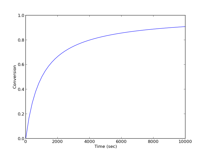
You can read off of this figure to find the time required to achieve a particular conversion.

org-mode source

Discuss on Twitter

Numerical propagation of errors

Posted February 16, 2013 at 09:00 AM | categories: statistics | tags:

Updated March 07, 2013 at 08:46 AM

Matlab post

Propagation of errors is essential to understanding how the uncertainty in a parameter affects computations that use that parameter. The uncertainty propagates by a set of rules into your solution. These rules are not easy to remember, or apply to complicated situations, and are only approximate for equations that are nonlinear in the parameters.

We will use a Monte Carlo simulation to illustrate error propagation. The idea is to generate a distribution of possible parameter values, and to evaluate your equation for each parameter value. Then, we perform statistical analysis on the results to determine the standard error of the results.

We will assume all parameters are defined by a normal distribution with known mean and standard deviation.

1 Addition and subtraction

import numpy as np
import matplotlib.pyplot as plt

N = 1e6 # number of samples of parameters

A_mu = 2.5; A_sigma = 0.4
B_mu = 4.1; B_sigma = 0.3

A = np.random.normal(A_mu, A_sigma, size=(1, N))
B = np.random.normal(B_mu, B_sigma, size=(1, N))

p = A + B
m = A - B

print np.std(p)
print np.std(m)

print np.sqrt(A_sigma**2 + B_sigma**2) # the analytical std dev

>>> >>> >>> >>> >>> >>> >>> >>> >>> >>> >>> >>> >>> 0.500505424616
0.500113385681
>>> 0.5

2 Multiplication

F_mu = 25.0; F_sigma = 1;
x_mu = 6.4; x_sigma = 0.4;

F = np.random.normal(F_mu, F_sigma, size=(1, N))
x = np.random.normal(x_mu, x_sigma, size=(1, N))

t = F * x
print np.std(t)
print np.sqrt((F_sigma / F_mu)**2 + (x_sigma / x_mu)**2) * F_mu * x_mu

>>> >>> >>> >>> >>> >>> 11.8900166284
11.8726576637

3 Division

This is really like multiplication: F / x = F * (1 / x).

d = F / x
print np.std(d)
print np.sqrt((F_sigma / F_mu)**2 + (x_sigma / x_mu)**2) * F_mu / x_mu

0.293757533168
0.289859806243

4 exponents

This rule is different than multiplication (A^2 = A*A) because in the previous examples we assumed the errors in A and B for A*B were uncorrelated. in A*A, the errors are not uncorrelated, so there is a different rule for error propagation.

t_mu = 2.03; t_sigma = 0.01*t_mu; # 1% error
A_mu = 16.07; A_sigma = 0.06;

t = np.random.normal(t_mu, t_sigma, size=(1, N))
A = np.random.normal(A_mu, A_sigma, size=(1, N))

# Compute t^5 and sqrt(A) with error propagation
print np.std(t**5)
print (5 * t_sigma / t_mu) * t_mu**5

>>> >>> >>> >>> >>> ... 1.72454836176
1.72365440621

print np.std(np.sqrt(A))
print 1.0 / 2.0 * A_sigma / A_mu * np.sqrt(A_mu)

0.00748903477329
0.00748364738749

5 the chain rule in error propagation

let v = v0 + a*t, with uncertainties in vo,a and t

vo_mu = 1.2; vo_sigma = 0.02;
a_mu = 3.0;  a_sigma  = 0.3;
t_mu = 12.0; t_sigma  = 0.12;

vo = np.random.normal(vo_mu, vo_sigma, (1, N))
a = np.random.normal(a_mu, a_sigma, (1, N))
t = np.random.normal(t_mu, t_sigma, (1, N))

v = vo + a*t

print np.std(v)
print np.sqrt(vo_sigma**2 + t_mu**2 * a_sigma**2 + a_mu**2 * t_sigma**2)

>>> >>> >>> >>> >>> >>> >>> >>> >>> 3.62232509326
3.61801050303

6 Summary

You can numerically perform error propagation analysis if you know the underlying distribution of errors on the parameters in your equations. One benefit of the numerical propogation is you do not have to remember the error propagation rules, and you directly look at the distribution in nonlinear cases. Some limitations of this approach include

You have to know the distribution of the errors in the parameters
You have to assume the errors in parameters are uncorrelated.

org-mode source

Discuss on Twitter

Numerical propogation of errors

Posted February 16, 2013 at 09:00 AM | categories: statistics | tags:

Updated February 27, 2013 at 02:36 PM

Matlab post

Propagation of errors is essential to understanding how the uncertainty in a parameter affects computations that use that parameter. The uncertainty propogates by a set of rules into your solution. These rules are not easy to remember, or apply to complicated situations, and are only approximate for equations that are nonlinear in the parameters.

We will use a Monte Carlo simulation to illustrate error propogation. The idea is to generate a distribution of possible parameter values, and to evaluate your equation for each parameter value. Then, we perform statistical analysis on the results to determine the standard error of the results.

We will assume all parameters are defined by a normal distribution with known mean and standard deviation.

1 Addition and subtraction

import numpy as np
import matplotlib.pyplot as plt

N = 1e6 # number of samples of parameters

A_mu = 2.5; A_sigma = 0.4
B_mu = 4.1; B_sigma = 0.3

A = np.random.normal(A_mu, A_sigma, size=(1, N))
B = np.random.normal(B_mu, B_sigma, size=(1, N))

p = A + B
m = A - B

print np.std(p)
print np.std(m)

print np.sqrt(A_sigma**2 + B_sigma**2) # the analytical std dev

>>> >>> >>> >>> >>> >>> >>> >>> >>> >>> >>> >>> >>> 0.500505424616
0.500113385681
>>> 0.5

2 Multiplication

F_mu = 25.0; F_sigma = 1;
x_mu = 6.4; x_sigma = 0.4;

F = np.random.normal(F_mu, F_sigma, size=(1, N))
x = np.random.normal(x_mu, x_sigma, size=(1, N))

t = F * x
print np.std(t)
print np.sqrt((F_sigma / F_mu)**2 + (x_sigma / x_mu)**2) * F_mu * x_mu

>>> >>> >>> >>> >>> >>> 11.8900166284
11.8726576637

3 Division

This is really like multiplication: F / x = F * (1 / x).

d = F / x
print np.std(d)
print np.sqrt((F_sigma / F_mu)**2 + (x_sigma / x_mu)**2) * F_mu / x_mu

0.293757533168
0.289859806243

4 exponents

t_mu = 2.03; t_sigma = 0.01*t_mu; # 1% error
A_mu = 16.07; A_sigma = 0.06;

t = np.random.normal(t_mu, t_sigma, size=(1, N))
A = np.random.normal(A_mu, A_sigma, size=(1, N))

# Compute t^5 and sqrt(A) with error propogation
print np.std(t**5)
print (5 * t_sigma / t_mu) * t_mu**5

>>> >>> >>> >>> >>> ... 1.72454836176
1.72365440621

print np.std(np.sqrt(A))
print 1.0 / 2.0 * A_sigma / A_mu * np.sqrt(A_mu)

0.00748903477329
0.00748364738749

5 the chain rule in error propogation

let v = v0 + a*t, with uncertainties in vo,a and t

vo_mu = 1.2; vo_sigma = 0.02;
a_mu = 3.0;  a_sigma  = 0.3;
t_mu = 12.0; t_sigma  = 0.12;

vo = np.random.normal(vo_mu, vo_sigma, (1, N))
a = np.random.normal(a_mu, a_sigma, (1, N))
t = np.random.normal(t_mu, t_sigma, (1, N))

v = vo + a*t

print np.std(v)
print np.sqrt(vo_sigma**2 + t_mu**2 * a_sigma**2 + a_mu**2 * t_sigma**2)

>>> >>> >>> >>> >>> >>> >>> >>> >>> 3.62232509326
3.61801050303

6 Summary

You can numerically perform error propogation analysis if you know the underlying distribution of errors on the parameters in your equations. One benefit of the numerical propogation is you do not have to remember the error propogation rules, and you directly look at the distribution in nonlinear cases. Some limitations of this approach include

You have to know the distribution of the errors in the parameters
You have to assume the errors in parameters are uncorrelated.

org-mode source

Discuss on Twitter

Plane Poiseuille flow - BVP solve by shooting method

Posted February 15, 2013 at 09:00 AM | categories: bvp | tags: fluids

Updated March 08, 2013 at 10:08 AM

Matlab post

One approach to solving BVPs is to use the shooting method. The reason we cannot use an initial value solver for a BVP is that there is not enough information at the initial value to start. In the shooting method, we take the function value at the initial point, and guess what the function derivatives are so that we can do an integration. If our guess was good, then the solution will go through the known second boundary point. If not, we guess again, until we get the answer we need. In this example we repeat the pressure driven flow example, but illustrate the shooting method.

In the pressure driven flow of a fluid with viscosity $\mu$ between two stationary plates separated by distance $d$ and driven by a pressure drop $\Delta P/\Delta x$, the governing equations on the velocity $u$ of the fluid are (assuming flow in the x-direction with the velocity varying only in the y-direction):

$$\frac{\Delta P}{\Delta x} = \mu \frac{d^2u}{dy^2}$$

with boundary conditions $u(y=0) = 0$ and $u(y=d) = 0$, i.e. the no-slip condition at the edges of the plate.

we convert this second order BVP to a system of ODEs by letting $u_1 = u$, $u_2 = u_1'$ and then $u_2' = u_1''$. This leads to:

$\frac{d u_1}{dy} = u_2$

$\frac{d u_2}{dy} = \frac{1}{\mu}\frac{\Delta P}{\Delta x}$

with boundary conditions $u_1(y=0) = 0$ and $u_1(y=d) = 0$.

for this problem we let the plate separation be d=0.1, the viscosity $\mu = 1$, and $\frac{\Delta P}{\Delta x} = -100$.

1 First guess

We need u_1(0) and u_2(0), but we only have u_1(0). We need to guess a value for u_2(0) and see if the solution goes through the u_2(d)=0 boundary value.

import numpy as np
from scipy.integrate import odeint
import matplotlib.pyplot as plt

d = 0.1 # plate thickness

def odefun(U, y):
    u1, u2 = U
    mu = 1
    Pdrop = -100
    du1dy = u2
    du2dy = 1.0 / mu * Pdrop
    return [du1dy, du2dy]

u1_0 = 0 # known
u2_0 = 1 # guessed

dspan = np.linspace(0, d)

U = odeint(odefun, [u1_0, u2_0], dspan)

plt.plot(dspan, U[:,0])
plt.plot([d],[0], 'ro')
plt.xlabel('d')
plt.ylabel('$u_1$')
plt.savefig('images/bvp-shooting-1.png')

Here we have undershot the boundary condition. Let us try a larger guess.

2 Second guess

import numpy as np
from scipy.integrate import odeint
import matplotlib.pyplot as plt

d = 0.1 # plate thickness

def odefun(U, y):
    u1, u2 = U
    mu = 1
    Pdrop = -100
    du1dy = u2
    du2dy = 1.0 / mu * Pdrop
    return [du1dy, du2dy]

u1_0 = 0 # known
u2_0 = 10 # guessed

dspan = np.linspace(0, d)

U = odeint(odefun, [u1_0, u2_0], dspan)

plt.plot(dspan, U[:,0])
plt.plot([d],[0], 'ro')
plt.xlabel('d')
plt.ylabel('$u_1$')
plt.savefig('images/bvp-shooting-2.png')

Now we have clearly overshot. Let us now make a function that will iterate for us to find the right value.

3 Let fsolve do the work

import numpy as np
from scipy.integrate import odeint
from scipy.optimize import fsolve
import matplotlib.pyplot as plt

d = 0.1 # plate thickness
Pdrop = -100
mu = 1

def odefun(U, y):
    u1, u2 = U
    du1dy = u2
    du2dy = 1.0 / mu * Pdrop
    return [du1dy, du2dy]

u1_0 = 0 # known
dspan = np.linspace(0, d)

def objective(u2_0):
    dspan = np.linspace(0, d)
    U = odeint(odefun, [u1_0, u2_0], dspan)
    u1 = U[:,0]
    return u1[-1]

u2_0, = fsolve(objective, 1.0)

# now solve with optimal u2_0
U = odeint(odefun, [u1_0, u2_0], dspan)

plt.plot(dspan, U[:,0], label='Numerical solution')
plt.plot([d],[0], 'ro')

# plot an analytical solution
u = -(Pdrop) * d**2 / 2 / mu * (dspan / d - (dspan / d)**2)
plt.plot(dspan, u, 'r--', label='Analytical solution')


plt.xlabel('d')
plt.ylabel('$u_1$')
plt.legend(loc='best')
plt.savefig('images/bvp-shooting-3.png')

You can see the agreement is excellent!

This also seems like a useful bit of code to not have to reinvent regularly, so it has been added to pycse as BVP_sh. Here is an example usage.

from pycse import BVP_sh
import matplotlib.pyplot as plt

d = 0.1 # plate thickness
Pdrop = -100
mu = 1

def odefun(U, y):
    u1, u2 = U
    du1dy = u2
    du2dy = 1.0 / mu * Pdrop
    return [du1dy, du2dy]

x1 = 0.0; alpha = 0.0
x2 = 0.1; beta = 0.0
init = 2.0 # initial guess of slope at x=0

X,Y = BVP_sh(odefun, x1, x2, alpha, beta, init)
plt.plot(X, Y[:,0])
plt.ylim([0, 0.14])

# plot an analytical solution
u = -(Pdrop) * d**2 / 2 / mu * (X / d - (X / d)**2)
plt.plot(X, u, 'r--', label='Analytical solution')
plt.savefig('images/bvp-shooting-4.png')
plt.show()

org-mode source

Discuss on Twitter

The equal area method for the van der Waals equation

Posted February 15, 2013 at 09:00 AM | categories: plotting | tags: thermodynamics

Updated September 25, 2013 at 09:13 AM

1. Compute areas

Matlab post

When a gas is below its Tc the van der Waal equation oscillates. In the portion of the isotherm where $\partial P_R/\partial V_r > 0$, the isotherm fails to describe real materials, which phase separate into a liquid and gas in this region.

Maxwell proposed to replace this region by a flat line, where the area above and below the curves are equal. Today, we examine how to identify where that line should be.

import numpy as np
import matplotlib.pyplot as plt

Tr = 0.9 # A Tr below Tc:  Tr = T/Tc
# analytical equation for Pr. This is the reduced form of the van der Waal
# equation.
def Prfh(Vr):
    return  8.0 / 3.0 * Tr / (Vr - 1.0 / 3.0) - 3.0 / (Vr**2)

Vr = np.linspace(0.5, 4, 100)  # vector of reduced volume
Pr = Prfh(Vr)                 # vector of reduced pressure

plt.plot(Vr,Pr)
plt.ylim([0, 2])
plt.xlabel('$V_R$')
plt.ylabel('$P_R$')
plt.savefig('images/maxwell-eq-area-1.png')

>>> >>> >>> >>> >>> >>> ... ... ... ... >>> >>> >>> >>> [<matplotlib.lines.Line2D object at 0x042FDAF0>]
(0, 2)
<matplotlib.text.Text object at 0x04237CB0>
<matplotlib.text.Text object at 0x042DC030>

The idea is to pick a Pr and draw a line through the EOS. We want the areas between the line and EOS to be equal on each side of the middle intersection. Let us draw a line on the figure at y = 0.65.

y = 0.65

plt.plot([0.5, 4.0], [y, y], 'k--')
plt.savefig('images/maxwell-eq-area-2.png')

>>> [<matplotlib.lines.Line2D object at 0x042FDCD0>]

To find the areas, we need to know where the intersection of the vdW eqn with the horizontal line. This is the same as asking what are the roots of the vdW equation at that Pr. We need all three intersections so we can integrate from the first root to the middle root, and then the middle root to the third root. We take advantage of the polynomial nature of the vdW equation, which allows us to use the roots command to get all the roots at once. The polynomial is $V_R^3 - \frac{1}{3}(1+8 T_R/P_R) + 3/P_R - 1/P_R = 0$. We use the coefficients t0 get the roots like this.

vdWp = [1.0, -1. / 3.0 * (1.0 + 8.0 * Tr / y), 3.0 / y, - 1.0 / y]
v = np.roots(vdWp)
v.sort()
print v

plt.plot(v[0], y, 'bo', v[1], y, 'bo', v[2], y, 'bo')
plt.savefig('images/maxwell-eq-area-3.png')

>>> >>> [ 0.60286812  1.09743234  2.32534056]
>>> [<matplotlib.lines.Line2D object at 0x0439C570>, <matplotlib.lines.Line2D object at 0x043933B0>, <matplotlib.lines.Line2D object at 0x04393CB0>]

1 Compute areas

for A1, we need the area under the line minus the area under the vdW curve. That is the area between the curves. For A2, we want the area under the vdW curve minus the area under the line. The area under the line between root 2 and root 1 is just the width (root2 - root1)*y

from scipy.integrate import quad

A1, e1 = (v[1] - v[0]) * y - quad(Prfh,  v[0], v[1])
A2, e2 = quad(Prfh, v[1], v[2]) - (v[2] - v[1])* y 

print A1, A2
print e1, e2  # interesting these look so large

>>> >>> >>> >>> 0.063225945606 0.0580212098122
0.321466743765 -0.798140339268

from scipy.optimize import fsolve

def equal_area(y):
    Tr = 0.9
    vdWp = [1, -1.0 / 3 * ( 1.0 + 8.0 * Tr / y), 3.0 / y,  -1.0 / y]
    v = np.roots(vdWp)
    v.sort()
    A1 = (v[1] - v[0]) * y - quad(Prfh, v[0], v[1])
    A2 = quad(Prfh, v[1], v[2]) - (v[2] - v[1]) * y
    return  A1 - A2

y_eq, = fsolve(equal_area, 0.65)
print y_eq

Tr = 0.9
vdWp = [1, -1.0 / 3 * ( 1.0 + 8.0 * Tr / y_eq), 3.0 / y_eq,  -1.0 / y_eq]
v = np.roots(vdWp)
v.sort()

A1, e1 = (v[1] - v[0]) * y_eq - quad(Prfh,  v[0], v[1])
A2, e2 = quad(Prfh, v[1], v[2]) - (v[2] - v[1]) * y_eq

print A1, A2

>>> ... ... ... ... ... ... ... ... >>> >>> 0.646998351872
>>> >>> >>> >>> >>> >>> >>> >>> >>> 0.0617526473994 0.0617526473994

Now let us plot the equal areas and indicate them by shading.

fig = plt.gcf()
ax = fig.add_subplot(111)

ax.plot(Vr,Pr)

hline = np.ones(Vr.size) * y_eq

ax.plot(Vr, hline)
ax.fill_between(Vr, hline, Pr, where=(Vr >= v[0]) & (Vr <= v[1]), facecolor='gray')
ax.fill_between(Vr, hline, Pr, where=(Vr >= v[1]) & (Vr <= v[2]), facecolor='gray')

plt.text(v[0], 1, 'A1 = {0}'.format(A1))
plt.text(v[2], 1, 'A2 = {0}'.format(A2))
plt.xlabel('$V_R$')
plt.ylabel('$P_R$')
plt.title('$T_R$ = 0.9')

plt.savefig('images/maxwell-eq-area-4.png')
plt.savefig('images/maxwell-eq-area-4.svg')

>>> >>> [<matplotlib.lines.Line2D object at 0x043939D0>]
>>> >>> >>> [<matplotlib.lines.Line2D object at 0x043A7230>]
<matplotlib.collections.PolyCollection object at 0x047ADE70>
<matplotlib.collections.PolyCollection object at 0x047ADAB0>
>>> <matplotlib.text.Text object at 0x0438E730>
<matplotlib.text.Text object at 0x047B7930>
<matplotlib.text.Text object at 0x04237CB0>
<matplotlib.text.Text object at 0x042DC030>
<matplotlib.text.Text object at 0x042EBCD0>

org-mode source

Discuss on Twitter

« Previous Page -- Next Page »

The Kitchin Research Group

Chemical Engineering at Carnegie Mellon University

Integrating the batch reactor mole balance

Numerical propagation of errors

1 Addition and subtraction

2 Multiplication

3 Division

4 exponents

5 the chain rule in error propagation

6 Summary

Numerical propogation of errors

1 Addition and subtraction

2 Multiplication

3 Division

4 exponents

5 the chain rule in error propogation

6 Summary

Plane Poiseuille flow - BVP solve by shooting method

1 First guess

2 Second guess

3 Let fsolve do the work

The equal area method for the van der Waals equation

Table of Contents

1 Compute areas