Plug flow reactor with a pressure drop

| categories: ode | tags: reaction engineering, fluids

If there is a pressure drop in a plug flow reactor, 1 there are two equations needed to determine the exit conversion: one for the conversion, and one from the pressure drop.

\begin{eqnarray} \frac{dX}{dW} &=& \frac{k'}{F_A0} \left ( \frac{1-X}{1 + \epsilon X} \right) y\\ \frac{dX}{dy} &=& -\frac{\alpha (1 + \epsilon X)}{2y} \end{eqnarray}

Here is how to integrate these equations numerically in python.

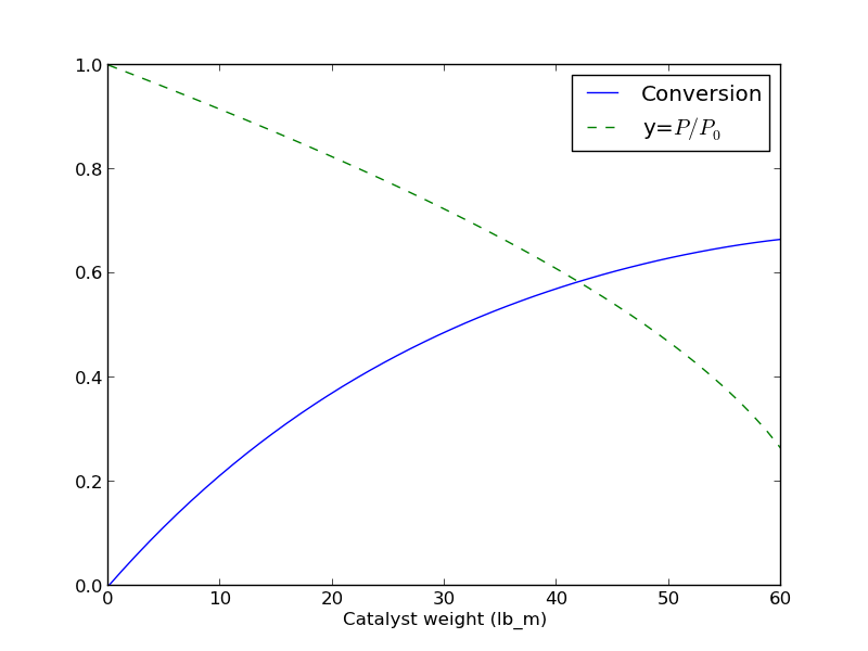
import numpy as np
from scipy.integrate import odeint
import matplotlib.pyplot as plt

kprime = 0.0266
Fa0 = 1.08
alpha = 0.0166
epsilon = -0.15

def dFdW(F, W):
    'set of ODEs to integrate'
    X = F[0]
    y = F[1]
    dXdW = kprime / Fa0 * (1-X) / (1 + epsilon*X) * y
    dydW = -alpha * (1 + epsilon * X) / (2 * y)
    return [dXdW, dydW]

Wspan = np.linspace(0,60)
X0 = 0.0
y0 = 1.0
F0 = [X0, y0]
sol = odeint(dFdW, F0, Wspan)

# now plot the results
plt.plot(Wspan, sol[:,0], label='Conversion')
plt.plot(Wspan, sol[:,1], 'g--', label='y=$P/P_0$')
plt.legend(loc='best')
plt.xlabel('Catalyst weight (lb_m)')
plt.savefig('images/2013-01-08-pdrop.png')

Here is the resulting figure.

Copyright (C) 2013 by John Kitchin. See the License for information about copying.

org-mode source

Discuss on Twitter

Linear regression with confidence intervals.

| categories: data analysis, linear regression, confidence interval | tags:

Matlab post Fit a fourth order polynomial to this data and determine the confidence interval for each parameter. Data from example 5-1 in Fogler, Elements of Chemical Reaction Engineering.

We want the equation \(Ca(t) = b0 + b1*t + b2*t^2 + b3*t^3 + b4*t^4\) fit to the data in the least squares sense. We can write this in a linear algebra form as: T*p = Ca where T is a matrix of columns [1 t t^2 t^3 t^4], and p is a column vector of the fitting parameters. We want to solve for the p vector and estimate the confidence intervals.

import numpy as np
from scipy.stats.distributions import  t

time = np.array([0.0, 50.0, 100.0, 150.0, 200.0, 250.0, 300.0])
Ca = np.array([50.0, 38.0, 30.6, 25.6, 22.2, 19.5, 17.4])*1e-3

T = np.column_stack([time**0, time, time**2, time**3, time**4])

p, res, rank, s = np.linalg.lstsq(T, Ca)
# the parameters are now in p

# compute the confidence intervals
n = len(Ca)
k = len(p)

sigma2 = np.sum((Ca - np.dot(T, p))**2) / (n - k)  # RMSE

C = sigma2 * np.linalg.inv(np.dot(T.T, T)) # covariance matrix
se = np.sqrt(np.diag(C)) # standard error

alpha = 0.05 # 100*(1 - alpha) confidence level

sT = t.ppf(1.0 - alpha/2.0, n - k) # student T multiplier
CI = sT * se

for beta, ci in zip(p, CI):
    print '{2: 1.2e} [{0: 1.4e} {1: 1.4e}]'.format(beta - ci, beta + ci, beta)

SS_tot = np.sum((Ca - np.mean(Ca))**2)
SS_err = np.sum((np.dot(T, p) - Ca)**2)

#  http://en.wikipedia.org/wiki/Coefficient_of_determination
Rsq = 1 - SS_err/SS_tot
print 'R^2 = {0}'.format(Rsq)

# plot fit
import matplotlib.pyplot as plt
plt.plot(time, Ca, 'bo', label='raw data')
plt.plot(time, np.dot(T, p), 'r-', label='fit')
plt.xlabel('Time')
plt.ylabel('Ca (mol/L)')
plt.legend(loc='best')
plt.savefig('images/linregress-conf.png')
 5.00e-02 [ 4.9680e-02  5.0300e-02]
-2.98e-04 [-3.1546e-04 -2.8023e-04]
 1.34e-06 [ 1.0715e-06  1.6155e-06]
-3.48e-09 [-4.9032e-09 -2.0665e-09]
 3.70e-12 [ 1.3501e-12  6.0439e-12]
R^2 = 0.999986967246

A fourth order polynomial fits the data well, with a good R^2 value. All of the parameters appear to be significant, i.e. zero is not included in any of the parameter confidence intervals. This does not mean this is the best model for the data, just that the model fits well.

Copyright (C) 2013 by John Kitchin. See the License for information about copying.

org-mode source

Discuss on Twitter

Basic statistics

| categories: statistics | tags:

Given several measurements of a single quantity, determine the average value of the measurements, the standard deviation of the measurements and the 95% confidence interval for the average.

This is a recipe for computing the confidence interval. The strategy is:

  1. compute the average
  2. Compute the standard deviation of your data
  3. Define the confidence interval, e.g. 95% = 0.95
  4. compute the student-t multiplier. This is a function of the confidence

interval you specify, and the number of data points you have minus 1. You subtract 1 because one degree of freedom is lost from calculating the average. The confidence interval is defined as ybar +- T_multiplier*std/sqrt(n).

import numpy as np
from scipy.stats.distributions import  t

y = [8.1, 8.0, 8.1]

ybar = np.mean(y)
s = np.std(y)

ci = 0.95
alpha = 1.0 - ci

n = len(y)
T_multiplier = t.ppf(1-alpha/2.0, n-1)

ci95 = T_multiplier * s / np.sqrt(n-1)

print [ybar - ci95, ybar + ci95]
[7.9232449090029595, 8.210088424330376]

We are 95% certain the next measurement will fall in the interval above.

Copyright (C) 2013 by John Kitchin. See the License for information about copying.

org-mode source

Discuss on Twitter

Introduction to statistical data analysis

| categories: statistics | tags:

Matlab post

Given several measurements of a single quantity, determine the average value of the measurements, the standard deviation of the measurements and the 95% confidence interval for the average.

import numpy as np

y = [8.1, 8.0, 8.1]

ybar = np.mean(y)
s = np.std(y, ddof=1)

print ybar, s
>>> >>> >>> >>> >>> >>> 8.06666666667 0.057735026919

Interesting, we have to specify the divisor in numpy.std by the ddof argument. The default for this in Matlab is 1, the default for this function is 0.

Here is the principle of computing a confidence interval.

  1. compute the average
  2. Compute the standard deviation of your data
  3. Define the confidence interval, e.g. 95% = 0.95
  4. compute the student-t multiplier. This is a function of the confidence interval you specify, and the number of data points you have minus 1. You subtract 1 because one degree of freedom is lost from calculating the average.

The confidence interval is defined as ybar +- T_multiplier*std/sqrt(n).

from scipy.stats.distributions import  t
ci = 0.95
alpha = 1.0 - ci

n = len(y)
T_multiplier = t.ppf(1.0 - alpha / 2.0, n - 1)

ci95 = T_multiplier * s / np.sqrt(n)

print 'T_multiplier = {0}'.format(T_multiplier)
print 'ci95 = {0}'.format(ci95)
print 'The true average is between {0} and {1} at a 95% confidence level'.format(ybar - ci95, ybar + ci95)
>>> >>> >>> >>> >>> >>> >>> >>> T_multiplier = 4.30265272991
ci95 = 0.143421757664
The true average is between 7.923244909 and 8.21008842433 at a 95% confidence level

Copyright (C) 2013 by John Kitchin. See the License for information about copying.

org-mode source

Discuss on Twitter

Solving CSTR design equations

| categories: nonlinear algebra | tags: reaction engineering

Given a continuously stirred tank reactor with a volume of 66,000 dm^3 where the reaction \(A \rightarrow B\) occurs, at a rate of \(-r_A = k C_A^2\) (\(k=3\) L/mol/h), with an entering molar flow of F_{A0} = 5 mol/h and a volumetric flowrate of 10 L/h, what is the exit concentration of A?

From a mole balance we know that at steady state \(0 = F_{A0} - F_A + V r_A\). That equation simply states the sum of the molar flow of A in in minus the molar flow of A out plus the molar rate A is generated is equal to zero at steady state. This is directly the equation we need to solve. We need the following relationship:

  1. \(F_A = v0 C_A\)
from scipy.optimize import fsolve

Fa0 = 5.0
v0 = 10.

V = 66000.0  # reactor volume L^3
k = 3.0      # rate constant L/mol/h

def func(Ca):
    "Mole balance for a CSTR. Solve this equation for func(Ca)=0"
    Fa = v0 * Ca     # exit molar flow of A
    ra = -k * Ca**2  # rate of reaction of A L/mol/h
    return Fa0 - Fa + V * ra

# CA guess that that 90 % is reacted away
CA_guess = 0.1 * Fa0 / v0
CA_sol, = fsolve(func, CA_guess)

print 'The exit concentration is {0} mol/L'.format(CA_sol)
The exit concentration is 0.005 mol/L

It is a little confusing why it is necessary to put a comma after the CA_sol in the fsolve command. If you do not put it there, you get brackets around the answer.

Copyright (C) 2013 by John Kitchin. See the License for information about copying.

org-mode source

Discuss on Twitter
« Previous Page -- Next Page »